
图论
基本概念
图: 点用边连起来就叫做图,严格一样上讲,图是一种数据结构,定义为:\(graph=(V,E)\)。
\(V\)是一个非空有限集合,代表顶点(结点),\(E\)代表边的集合。
有向图: 图的边有方向,只能按箭头方向从一点到另一点。(a)是一个有向图
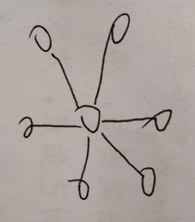
无向图: 图的边没有方向,可以双向。(b)是一个无向图

结点的度: 无向图中与结点相连的边的数目,称为结点的度。

结点的入度: 在有向图中,以这个结点为终点的有向边的数目。
结点的出度: 在有向图中,以这个结点为起点的有向边的数目。

权值: 边的“费用”,可以形象的理解为边的长度。
回路: 起点和终点相同的路径,称为回路,或“环”
完全图: 一个\(n\)阶的完全无向图含有\(n*(n-1)/2\)条边;一个\(n\)阶的完全有向图含有\(n*(n-1)\)条边。
稠密图: 一个边数接近完全图的图。
稀疏图: 一个边数远远少于完全图的图。
无向完全图: 有\(n*(n-1)/2\)条边的无向图
有向完全图: 有\(n*(n-1)\)条边的有向图

权: 与图的边或弧相关的数。
网: 带权的图


子图: 对于图\(G = (V, E)\),\(G' = (V', E')\),若存在\(V'\)是\(V\)的子集,\(E'\)是\(E\)的子集,则称图\(G'\)是'G'的一个子图


邻接点: 对于无向图\(G = (V, E)\),如果边\((v_1, v_2)∈E\),则称顶点\(v_1\)和\(v_2\)互为邻接点;边\((v_1, v_2)\)依附于顶点\(v_1\)和\(v_2\),或者说\(v_1\)和\(v_2\)相关联。
一条路径: 由图\(G\)中顶点\(V_i\)经过若干个顶点总可到达\(V_j\),则称由\(V_i\)经过的顶点序列到\(V_j\)为\(V_i\)到\(V_j\)的一条路径。
如上图所示:\(V_1-V_3-V_4\)是\(V_1\)到\(V_4\)的一条路径,同理:\(V_1-V_2-V_3-V_4\)也是\(V_1\)到\(V_4\)的一条路径。
路径长度: 路径上边的数目。
简单路径: 一条路径上的顶点除起点和终点可相同外,其它顶点都不相同。
例如:下图中的\(V_1-V_3-V_4\)、\(V_1-V_2-V_3-V_4\)、\(V_1-V_4\)均为简单路径。

回路(环):起始顶点和终结顶点相同的路径。
例如:如上图所示:\(V_1-V_3-V_4-V_1\)、\(V_1-V_2-V_3-V_4-V_1\)均为环。
简单回路(简单环):除第一个顶点与最后一个顶点之外,其他顶点不重复出现的回路。
连通:在无向图中,如果从顶点\(v\)到顶点\(v'\)存在路径,则称\(v\)和\(v'\)是连通的。
连通图:无向图\(G\)中如果任意两个顶点\(v_i, v_j\)之间都是连通的,则称图\(G\)是连通图。
图的存储
邻接矩阵
数据结构
设图的结点个数为 \(n\),定义 \(n \times n\) 的二维数组 \(g[N][N]\),其中 \(g[i][j]\) 表示结点 \(i\) 到 \(j\) 的边权。
带权图的边权定义:
无权图的边权定义:
图示:

邻接矩阵表示:
初始化
对于带权图,常用
memset(g, 0x3f, sizeof(g));
对于无权图,常用
memset(g, 0, sizeof(g));
或直接定义全局变量即可
加边
添加一条边 \((from,to, w)\),其中\(from\)为起点,\(to\)为终点,\(w\)为边权(无权图取 \(w=1\))。
有向图的邻接矩阵更新
对应邻接矩阵 \(g[N][N]\) 的更新规则为:
无向图的邻接矩阵更新
无向图中边是双向的,需同时更新双向权值:
遍历节点s的邻接点
对于带权图:
const int INF = 0x3f3f3f3f;
for (int i = 1; i <= n; i++)
{
    if (g[s][i] < INF)
	{
        cout << i <<' ';
    }
}
对于无权图:
for (int i = 1; i <= n; i++)
{
    if (g[s][i] == 1)
	{
        cout << i <<' ';
    }
}
优缺点
空间复杂度:\(O(v^2)\)
优点:直观,容易理解,可以直接查看任意两点的关系。
缺点:对于稀疏图,会有很多空间根本没有利用。不能处理重边。要查询某一个顶点的所有边,要枚举V次。
链氏前向星
数据结构
用数组模拟邻接表,需要一个表头数组\(h[maxn]\),一个结构体数组\(e[maxm]\)
\(h[maxn]\)表示以\(i\)为起点的第一条边在\(e\)数组中的位置(下标)。
\(e[i]\)表示第\(i\)条边的信息
\(maxn\)表示最大点数量,\(maxm\)表示最大边数量
const int maxn = 510;
const int maxm = 100010;

// 注意两个数组的大小,h 大小为结点个数,e 大小为边数,如果是无向图要两倍
int h[maxn] = {}, tot = 0;	// 表头数组,当前加入的边的数量
struct edge
{
	int to, nxt, w;	//边的终点,同一起点的下一条边的位置,权值
}e[maxm];
图示:

初始化
tot = 0;
memset(head, -1, sizeof(head));
加边
加一条边\((from,to,w)\),其中起点为\(from\),终点为\(to\),权值为\(w\)(无权图权值为\(1\)即可,或不要\(w\)这个成员变量)
void addedge(int x, int y, int z)
{
	e[++tot].to = y;
	e[tot].w = z;
	e[tot].nxt = h[x];
	h[x] = tot;
}
对于有向图:
addedge(from, to, w);
对于无向图:
addedge(from, to, w);
addedge(to, from, w);
遍历结点 s 的邻接点
对于带权图:
cout << "s 的每条出边信息为:" << endl;
int to, w;
for (int i = h[s]; i != -1; i = e[i].nxt) {
    to = e[i].to;
    w = e[i].w;
    cout << "终点:" << to << " 边权:" << w << endl;
}
vector模拟邻接表
数据结构
用一个大小为\(n\)的\(vector\)数组\(edge[N]\)来维护每个节点的出边信息。
\(edge[i]\)保存以\(i\)为起点的每条出边的信息(终点和权值),其中每个元素为一个\(pair\),如果需要更多信息,可以定义结构体。
对于带权图
struct EDGE
{
    int to, w; // 边的终点to,边权w
};
vector<EDGE> edge[N]; // edge[i]存储i的所有出边信息
或
typedef pair<int, int> pii;
vector<pii> edge[N]; // 同上,只是用pair实现
对于无权图
vector<int> edge[N]; // edge[i]存储i的所有邻接点
初始化
对于单组测试数据,直接定义全局变量即可,对于多组测试数据,每次要清空\(vector\)
for (int i = 1; i <= n; i++)
{	//n 为图中结点个数
    edge[i].clear();
}
加边
对于无权有向图,加入一条边\((from,to)\)
edge[from].push_back(to);
对于无权无向图,加入一条边\((from,to)\)
edge[from].push_back(to);
edge[to].push_back(from);
对于带权有向图,加入一条边\((from,to,w)\)
edge[from].push_back(Node{to, w}); // 结构体实现
edge[from].push_back(make_pair(to, w)); // pair实现
或
// c++11加入了emplace_back()函数,可以略微提升时间和空间的效率
edge[from].emplace_back(Node{to, w}); // 结构体实现
edge[from].emplace_back(make_pair(to, w)); // pair实现
对于带权无向图,加入一条边\((from,to,w)\)
// 结构体实现
edge[from].push_back(Node{to, w});
edge[to].push_back(Node{from, w});
// pair实现
edge[from].push_back(make_pair(to, w));
edge[to].push_back(make_pair(from, w));
或
// c++11加入了emplace_back()函数,可以略微提升时间和空间的效率
// 结构体实现
edge[from].emplace_back(Node{to, w});
edge[to].emplace_back(Node{from, w});
// pair实现
edge[from].emplace_back(make_pair(to, w));
edge[to].emplace_back(make_pair(from, w));
遍历结点\(s\)的邻接点
对于无权图:
printf("s 的邻接点:");
for (const auto &to : edge[s])
{
    printf("%d ", to);
}
对于带权图
// 结构体实现
int to, w;
printf("s 的邻接点:");
for (const auto &e : edge[s])
{
    to = e.to;
    w = e.w;
    printf("结点:%d 边权:%d\n", to, w);
}
或
// pair实现
int to, w;
printf("s 的邻接点:");
for (const auto &e : edge[s]) {
    to = e.first;
    w = e.second;
    printf("结点:%d 边权:%d\n", to, w);
}
图的遍历
DFS
概念说明
\(DFS\)全称是 Depth First Search,中文名是深度优先搜索,是一种用于遍历或搜索树或图的算法。所谓深度优先,就是说每次都尝试向更深的节点走。
该算法讲解时常常与\(BFS\)并列,但两者除了都能遍历图的连通块以外,用途完全不同,很少有能混用两种算法的情况。
\(DFS\)常常用来指代用递归函数实现的搜索,但实际上两者并不一样。
算法思想
\(DFS\)最显著的特征在于其递归调用自身。同时与\(BFS\)类似,\(DFS\)会对其访问过的点打上访问标记,在遍历图时跳过已打过标记的点,以确保每个点仅访问一次。
符合以上两条规则的函数,便是广义上的\(DFS\)
DFS(v) // v 可以是图中的一个顶点,也可以是抽象的概念,如 dp 状态等。
  在 v 上打访问标记
  for u in v 的相邻节点
    if u 没有打过访问标记 then
      DFS(u)
    end
  end
end
以上代码只包含了\(DFS\)必需的主要结构。实际的\(DFS\)会在以上代码基础上加入一些代码,利用\(DFS\)性质进行其他操作。
图示

深度优先遍历:\(v_1->v_2->v_4->v_5->v_3\)
深度优先遍历不唯一,跟存图顺序有关
复杂度
时间复杂度:\(O(n+m)\)
空间复杂度:\(O(n)\)
其中\(n\)表示点数,\(m\)表示边数
注:当图为一条链时,达到最坏空间复杂度\(O(n)\)
代码示例
DFS(邻接矩阵)
#include <bits/stdc++.h>
using namespace std;

const int maxn = 110;

int n = 0, m = 0;
int g[maxn][maxn] = {};
bool vis[maxn] = {};

void dfs(int x)
{
	vis[x] = true;
	printf("%d ", x);

	for(int i=1; i<=n; i++)
	{
		if(!vis[i] && g[x][i])
		{
			dfs(i);
		}
	}
}

int main()
{
	int x = 0, y = 0;

	scanf("%d%d", &n, &m);
	for(int i=1; i<=m; i++)
	{
		scanf("%d%d", &x, &y);
		g[x][y] = g[y][x] = 1;
	}

	dfs(1);

	return 0;
}
DFS(链氏前向星)
#include <bits/stdc++.h>
using namespace std;

const int maxn = 110;
const int maxm = 10010;

int n = 0, m = 0;
int h[maxn] = {}, tot = 0;
struct edge
{
	int to, nxt;
}e[maxm];
int v[maxn] = {};

void addedge(int x, int y)
{
	++tot;
	e[tot].to = y;
	e[tot].nxt = h[x];
	h[x] = tot;
}

void dfs(int x)
{
	printf("%d ", x);
	v[x] = true;

	for(int i=h[x]; i; i=e[i].nxt)
	{
		int y = e[i].to;
		if(!v[y])
		{
			dfs(y);
		}
	}
}

int main()
{
	int x = 0, y = 0;

	scanf("%d%d", &n, &m);
	for(int i=1; i<=m; i++)
	{
		scanf("%d%d", &x, &y);
		addedge(x, y);
		addedge(y, x);
	}

	dfs(1);

	return 0;
}
DFS(vector模拟邻接表)
#include <bits/stdc++.h>
using namespace std;

const int maxn = 110;

int n = 0, m = 0;
vector<int> e[maxn];
bool v[maxn] = {};

void dfs(int x)
{
	v[x] = true;
	printf("%d ", x);

	for(auto y : e[x])
	{
		if(!v[y])
		{
			dfs(y);
		}
	}
}

int main()
{
	int x = 0, y = 0;

	scanf("%d%d", &n, &m);
	for(int i=1; i<=m; i++)
	{
		scanf("%d%d", &x, &y);
		e[x].push_back(y);
		e[y].push_back(x);
	}

	dfs(1);

	return 0;
}
BFS
概念说明
\(BFS\)全称是Breadth First Search,中文名是宽度优先搜索,也叫广度优先搜索。
是图上最基础、最重要的搜索算法之一。
所谓宽度优先,就是每次都尝试访问同一层的节点,如果同一层都访问完了,再访问下一层。
这样做的结果是,\(BFS\)算法找到的路径是从起点开始的最短合法路径。换言之,这条路径所包含的边数最小。
在\(BFS\)结束时,每个节点都是通过从起点到该点的最短路径访问的。
算法过程可以看做是图上火苗传播的过程:最开始只是起点着火了,在每一时刻,有火的节点都向它相邻的所有节点传播火苗。
算法思想
我们用一个队列\(Q\)来记录要处理的节点,然后开一个布尔数组\(vis[]\)来标记是否已经访问过某个结点。
开始的时候,我们将所有节点的\(vis\)值设为\(0\),表示没有访问过;然后把起点\(s\)放入队列\(Q\)中并将\(vis[s]\)设为\(1\)。
之后,我们每次从队列\(Q\)中取出队首的结点\(u\),然后把与\(u\)相邻的所有节点\(v\)标记为已访问过并放入队列\(Q\)。
循环直至当队列\(Q\)为空,表示\(BFS\)结束。
在\(BFS\)的过程中,也可以记录一些额外的信息。\(d\)数组用于记录起点到某个节点的最短距离(要经过的最少边数),\(p\)数组记录是从哪个节点走到当前节点的。
有了\(d\)数组,可以方便地得到起点到一个节点的距离。
有了\(p\)数组,可以方便地还原出起点到一个点的最短路径。
图示

广度优先遍历:\(v_1->v_2->v_3->v_4->v_5->v_6->v_7->v_8\)
广度优先遍历不唯一,跟存图顺序有关
复杂度
时间复杂度:\(O(n+m)\)
空间复杂度:\(O(n)\)
其中\(n\)表示点数,\(m\)表示边数
代码示例
#include <bits/stdc++.h>
using namespace std;

const int maxn = 10010;

int n = 0, m = 0;
bool g[maxn][maxn] = {};
queue<int> q;
bool vis[maxn] = {};

void bfs(int x)
{
	q.push(x);
	vis[x] = true;

	while(!q.empty())
	{
		int t = q.front();
		printf("%d ", t);
		q.pop();

		for(int i=1; i<=n; i++)
		{
			if(g[t][i] && !vis[i])
			{
				q.push(i);
				vis[i] = true;
			}
		}
	}
}

int main()
{
	int x = 0, y = 0;

	scanf("%d%d", &n, &m);
	for(int i=1; i<=m; i++)
	{
		scanf("%d%d", &x, &y);
		g[x][y] = g[y][x] = 1;
	}

	bfs(1);

	return 0;
}
dfs序
\(dfs\)序是指\(dfs\)调用过程中访问的节点编号的序列。
\(dfs\)序不是唯一的
\(dfs\)序一般用于树状结构中,如图:
图中红色序号为每个点对应的\(dfs\)序序号,黑色序号为每个点默认的序号,我称之为节点序序号(下文同)
可见,\(dfs\)序如其名,\(dfs\)序序号是按照\(dfs\)顺序标记的,所以说给每个节点安排上\(dfs\)序序号也很简单,只要\(dfs\)的时候顺便标上就行了,\(dfs\)第多少次就给\(dfs\)到的点标为多少。
void dfs(int x)
{
	vis[x] = true;
	a[++cnt] = b[x];	//a数组记录的就是dfs序
	in[x] = cnt;	//记录以x为根节点的子树,在dfs序中开始的下标

	int v = 0;
	for(int i=head[x]; i; i=nxt[i])
	{
		v = to[i];
		if(vis[v]) continue;

		dfs(v);
	}
	out[x] = cnt;//记录以x为根节点的子树,在dfs序中结束的下标
}
\(dfs\)序的主要作用就是将一个子树变成序列上的一个连续区间。
还是以上图为例,
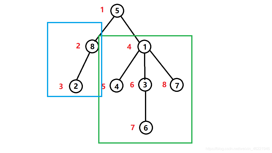
绿色子树可以通过\(dfs\)序序号表示出来,4~8;
红色子树表示为2~3;
显然,可以用一连续区间表示出来任意子树。
这样的变换可以解决类似“修改树上某点,输出子树和或者最大值最小值”等问题。
常常配合线段树或树状数组。
欧拉序
欧拉序长得跟\(dfs\)序相差无几
储存的则是从根节点开始,按照\(dfs\)的顺序经过所有点再绕回原点的路径
共存在两种欧拉序
欧拉序1
这一种欧拉序相当于是在\(dfs\)的时候,如果储存节点的栈变化一次,就把栈顶的节点编号记录下来,也就是说,每当访问完一个节点的子树,则需要返回一次该节点,再继续搜索该节点的其余子树,在树上的移动过程为
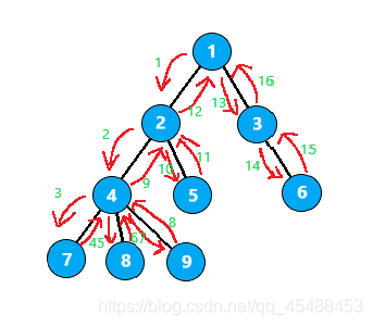
它的搜索顺序便是
1 2 4 7 4 8 4 9 4 2 5 2 1 3 6 3 1
搜索代码:
void euler_dfs1(int p)
{
    euler_order1[++pos]=p;
    vis[p]=true;
    for(int i:G[p])
        if(!vis[i])
        {
            euler_dfs1(i);
            euler_order1[++pos]=p; //与dfs序的差别,在搜索完一棵子树后就折返一次自己
        }
} //数组需要开2倍n大
欧拉序2
这一种欧拉序相当于是在\(dfs\)的时候,如果某个节点入栈,就把这个节点记录下来,直到后面的操作中这个节点出栈,再记录一次这个节点
也就是说,每个节点严格会在记录中出现两次,第一次是搜索到它的时候,第二次是它的子树完全被搜索完的时候
除根节点外,每个节点严格两个入度两个出度
在树上的移动过程为
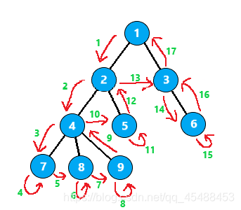
它的搜索顺序便是
1 2 4 7 7 8 8 9 9 4 5 5 2 3 6 6 3 1
可以发现,某个节点在顺序中出现的两次所围成的区间,就表示这个节点与它的子树
欧拉序 2 的搜索代码:
void euler_dfs2(int p)
{
    euler_order2[++pos]=p;
    vis[p]=true;
    for(int i:G[p])
        if(!vis[i])
            euler_dfs2(i);
    euler_order2[++pos]=p; //与dfs序的差别,在所有子树搜索完后再折返自己
} //数组需要开2倍n大
欧拉路&欧拉回路
概念
欧拉路: 经过图中每条边恰好一次的路径。
欧拉回路: 经过图中每条边恰好一次的回路。
注:每条边必需经过,且只经过一次,类似一笔画
奇点: 指跟这个点相连的边数目有奇数个的点。
定理1: 存在欧拉路的充要条件:图是连通的,有且只有2个奇点。
定理2: 存在欧拉回路的充要条件:图是连通的,有0个奇点。
两个定理的正确性是显而易见的,既然每条边都要经过一次,那么对于欧拉路,除了起点和终点外,每个点如果进入了一次,显然一定要出去一次,显然是偶点。对于欧拉回路,每个点进入和出去次数一定都是相等的,显然没有奇点。
求欧拉路的算法: 寻找节点的度为奇数的点,作为欧拉路的起点,执行深度优先遍历即可。
求欧拉回路的算法: 以任意一个点为起点,执行深度优先遍历即可
例题
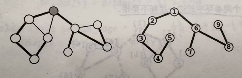
骑马修栅栏
题解:
1、要遍历图,先要存图,先看数据范围 边数<=1024,点数<=500,并且两点之间可能有多条路径,再加上输出结果时,要求点的字典序由小到大,因此想到邻接矩阵存图
2、该题就是一笔画问题,可能是欧拉路也可能是欧拉回路,要通过奇点数量来判断,注意该题的最小点不一定是1,也不一定连续,所以要求出最小点和最大点
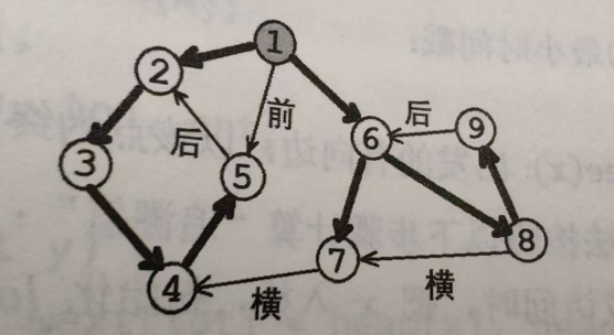
3、dfs遍历输出路径,正戏来了,输出路径有两种方式,见下面代码
void dfs(int x)
{
//	printf("%d\n", x);	//第一种方式

	//保证先搜顶点号小的,再搜顶点号大的
	for(int i=1; i<=n; i++)
	{
		if(g[x][i])
		{
			g[x][i]--;
			g[i][x]--;
			dfs(i);
		}
	}
	ans[++cnt] = x;		//第二种方式
}

//for(int i=cnt; i>=1; i--) printf("%d\n", ans[i]);

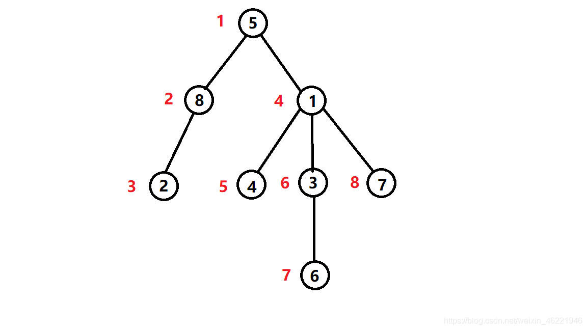
4、见上图,是欧拉路嵌套欧拉回路
如果采用第一种方式,从3这个节点,会贪心的输出4,然而看图可知,此时回不去了,无法走完那个欧拉回路,事实上dfs还在继续,最后输出1 2 3 4 5 6 3
如果采用第二种方式,在回溯的时候记录,我们也先得到4,4的搜索子树已经没了,4入栈,回到3,继续往5走,6,3,回到2,1,最后结果4 3 6 5 3 2 1,倒序输出1 2 3 5 6 3 4
基本上求路径的题目,回溯时记录会更加稳妥
#include <bits/stdc++.h>
using namespace std;

/*
考虑下面两个特殊情况
1、起点要从最小点开始,可能没有1号节点
2、基本上求路径的题目,回溯时记录会更加稳妥,详情见博客园
*/

const int maxn = 510;

int n = 0, m = 0; //n表示点数
int g[maxn][maxn] = {};
int du[maxn] = {};
int ans[maxn] = {}, cnt = 0;

void dfs(int x)
{
	//保证先搜顶点号小的,再搜顶点号大的
	for(int i=1; i<=n; i++)
	{
		if(g[x][i])
		{
			g[x][i]--;
			g[i][x]--;
			dfs(i);
		}
	}
	ans[++cnt] = x;
}

int main()
{
	int x = 0, y = 0;
	int st = maxn;	//最小的点

	scanf("%d", &m);
	for(int i=1; i<=m; i++)
	{
		scanf("%d%d", &x, &y);
		g[x][y]++;
		g[y][x]++;
		du[x]++;
		du[y]++;
		if(st > x) st = x;
		if(st > y) st = y;
		if(n < x) n = x;
		if(n < y) n = y;
	}

	//寻找节点的度为奇数的点,作为欧拉路的起点
	//没有度为奇数的点,则从st开始,求欧拉回路
	for(int i=1; i<=n; i++)
	{
		if(du[i] % 2 == 1)
		{
			st = i;
			break;
		}
	}

	dfs(st);

	for(int i=cnt; i>=1; i--) printf("%d\n", ans[i]);

	return 0;
}
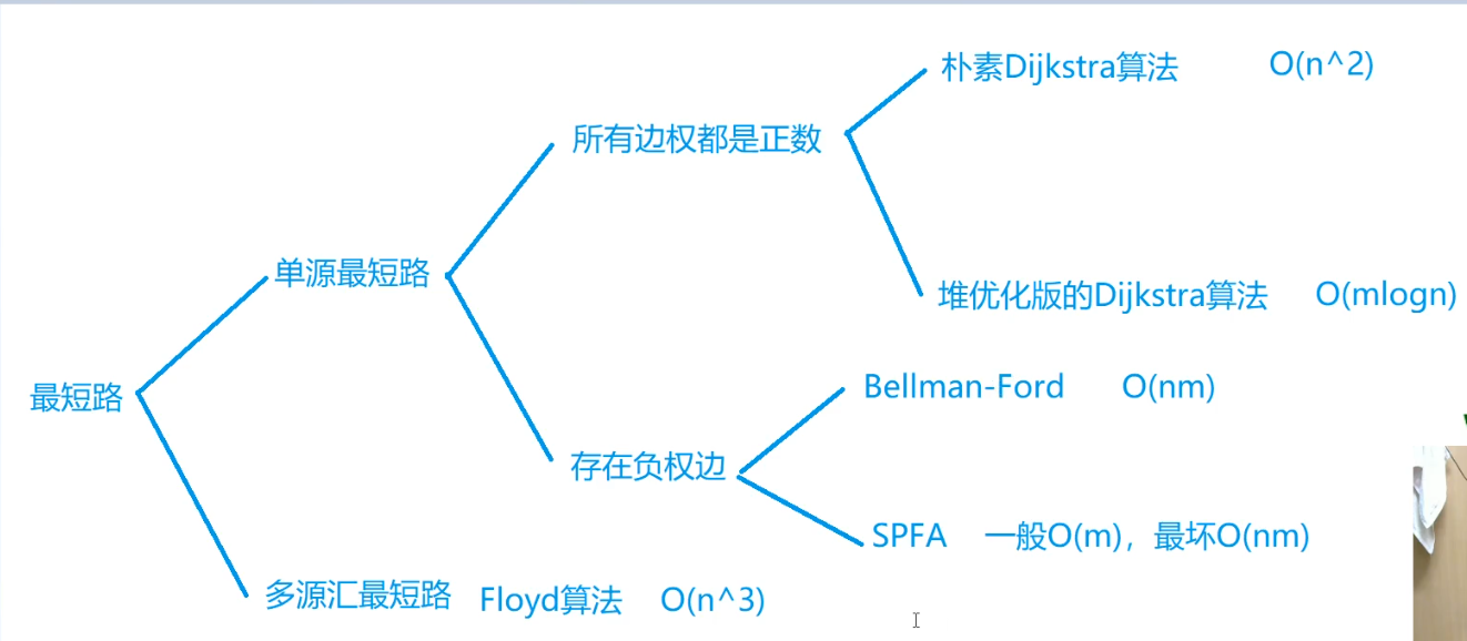
最短路
性质:
1、对于边权为正的图,任意两个节点之间的最短路,不会经过重复的点。
2、对于边权为正的图,任意两个节点之间的最短路,不会经过重复的边。
3、对于边权为正的图,任意两个节点之间的最短路,任意一条的节点数不会超过\(n\),边数不会超过\(n-1\)
ps:针对第3条的解释,一共就\(n\)个节点,所以最多经过\(n\)个节点;当节点数为\(n\)时,最多有\(n-1\)条边,如果再增加一条边,则要么经过重复边,要么构成环
Floyd
特点
用来求任意两个节点之间的最短路
负责度比较高,但常数小,容易实现(只有三个for)
适用于任何图,不管有向无向,边权正负,但是最短路必须存在(不能有负环)
实现
我们定义一个数组\(f[k][x][y]\),表示只允许经过节点\(1\)到\(k\)(也就是说,在子图\(V'=1,2,...,k\)中的路径,注意,\(x\)与\(y\)不一定在这个子图中),节点\(x\)到节点\(y\)的最短路长度。
显然,\(f[n][x][y]\)就是节点\(x\)到节点\(y\)的最短路长度(因为\(V'=1,2,...,n\)即为\(V\)本身,其表示的最短路径就是所求路径)。
接下来考虑如何求出\(f\)数组的值:
1、\(f[0][x][y]\):\(x\)与y的边权,或者0,或者+∞
(f[0][x][y]什么时候应该是+∞?当x与y间有直接相连的边的时候,为他们的边权;当x=y的时候为零,因为到本身的距离为零;当x与y没有直接相连的边的时候,为+∞)
2、\(f[k][x][y]=min(f[k-1][x][y], f[k-1][x][k] + f[k-1][k][y])\)
(f[k-1][x][y]为不经过k点的最短路径,而f[k-1][x][k] + f[k-1][k][y],为经过了k点的最短路)
这个做法的空间是\(O(n^3)\),我们需要依次增加问题规模(k从1到n),判断任意两点在当前问题规模下的最短路。
朴素版代码:
for(int k=1; k<=n; k++)
{
	for(int x=1; x<=n; x++)
	{
		for(int y=1; y<=n; y++)
		{
			f[k][x][y] = min(f[k-1][x][y], f[k-1][x][k] + f[k-1][k][y]);
		}
	}
}
优化:
因为第一维对结果无影响,我们发现数组的第一维是可以省略的,于是可以直接改成:
\(f[x][y] = min(f[x][y], f[x][k] + f[k][y])\)
证明:
对于给定的k,当更新f[k][x][y]时,涉及的元素总是来自f[k-1]数组的第k行和第k列。
然后我们可以发现,对于给定的k,当更新f[k][k][y]或f[k][x][k],总是不会发生数值更新,因为按照公式
f[k][k][y]=min(f[k-1][k][y], f[k-1][k][k] + f[k-1][k][y])
f[k-1][k][k]为0,因此这个值总是f[k-1][k][y],对于f[k][x][k]的证明类似。
因此,如果省略第一维,在给定的k下,每个元素的更新中使用到的元素都没有在这次迭代中更新,因此第一维的省略并不会影响结果。
优化后(最终)代码:
//初始化
memset(f, 0x3f, sizeof(f));
for(int i=1; i<=n; i++) f[i][i] = 0;

//算法结束后,dis[x][y]表示x到y的最短距离
void floyd()
{
	for(int k=1; k<=n; k++)
	{
		for(int i=1; i<=n; i++)
		{
			for(int j=1; j<=n; j++)
			{
				f[i][j] = min(f[i][j], f[i][k] + f[k][j]);
			}
		}
	}
}
注意: \(k\)一定要在最外层
反例:

如上图,f[1][4]=1;f[4][2]=3;f[4][3]=1;f[3][2]=1;其他不通,设为无限大
按k循环最内层来计算:
那么1,2节点的最短路径为:
\(min(f[1][2], f[1][3] + f[3][2], f[1][4] + f[4][2]) = 4\)(因为还没求到最小值f[1][3])
而且之后不再更新1,2节点的最短距离。
然而,实际上\(min(f[1][2]) = f[1][4] + f[4][3] + f[3][2] = 3\)
复杂度分析
时间复杂度是\(O(n^3)\)
空间复杂度\(O(n^2)\)
n表示点数
优缺点
优点:容易理解,可以算出任意两个节点之间的最短距离,代码编写简单
缺点:时间复杂度比较高,不适合计算大量数据
拓展应用
图的连通性问题
判断图中的两点是否连通
实现:把相连的两点间的距离设为f[i][j]=true,不相连的两点为f[i][j]=false,用floyed算法的变形
void floyd()
{
	for(int k=1; i<=n; k++)
	{
		for(int i=1; i<=n; i++)
		{
			for(int j=1; j<=n; j++)
			{
				f[i][j] = f[i][j] || (f[i][k] && f[k][j]);
			}
		}
	}
}
最后如果f[i][j]=true的话,那么就说明两点之间有路径连通。
有向图与无向图都适用。
优化: 可进一步用\(bitset\)优化,复杂度可以到\(O(n^3/w)\)
最小环问题
说明: 最小环就是指在一张图中找出一个环,使得这个环上的各条边的权值之和最小。在Floyed的同时,可以顺便算出最小环。
原理:
记录两点间的最短路为f[i][j],g[i][j]为边<i, j>的权值。
一个环中的最大节点为k(编号最大),与它相连的两个点为i,j,这个环的最短长度为
g[i][k]+g[k][j]+(i到j的路径中,所有节点编号都小于k的最短路径长度)
根据Floyed的原理,在最外层循环做了k-1次之后,f[i][j]则代表了i到j的路径中,所有节点编号都小于k的最短路径。
示例代码:
void floyd()
{
	for(int k=1; k<=n; k++)
	{
		for(int i=1; i<=k-1; i++)
		{
			for(int j=i+1; j<=k-1; j++)
			{
				ans = min(ans, f[i][j] + g[i][k] + g[k][j]);
			}
		}
		for(int i=1; i<=n; i++)
		{
			for(int j=1; j<=n; j++)
			{
				f[i][j] = min(f[i][j], f[i][k] + f[k][j]);
			}
		}
	}
}
上述代码中ans即为图中的最小环
例题
最短路径问题
#include <bits/stdc++.h>
using namespace std;

const int maxn = 110;

int n = 0, m = 0;
int a[maxn] = {}, b[maxn] = {};
double dis[maxn][maxn] = {};

void floyd()
{
	for(int k=1; k<=n; k++)
	{
		for(int i=1; i<=n; i++)
		{
			for(int j=1; j<=n; j++)
			{
				dis[i][j] = min(dis[i][j], dis[i][k]+dis[k][j]);
			}
		}
	}
}

int main()
{
	int x = 0, y = 0;
	scanf("%d", &n);
	for(int i=1; i<=n; i++) scanf("%d%d", &a[i], &b[i]);

	memset(dis, 0x7f, sizeof(dis));
	for(int i=1; i<=n; i++) dis[i][i] = 0;

	scanf("%d", &m);
	for(int i=1; i<=m; i++)
	{
		scanf("%d%d", &x, &y);
		dis[x][y] = dis[y][x] = sqrt((a[x]-a[y])*(a[x]-a[y]) + (b[x]-b[y])*(b[x]-b[y]));
	}

	floyd();

	scanf("%d%d", &x, &y);
	printf("%.2lf", dis[x][y]);

	return 0;
}
Dijkstra
\(Dijkstra\)算法由荷兰计算机科学家 E. W. Dijkstra 于 1956 年发现,1959 年公开发表。是一种求解非负权图上单源最短路径的算法。
核心思想:贪心

如上图,求结点①到其他点的最短路径,已知1->2的权值为5,1->3的权值为7,那么就可以贪心的认为节点①到节点②的最短路径就是5。
因为所有边权都为非负,所以从节点③再到节点②,假如有其他路径,也不可能是路径长度小于7
过程:
将节点分成两个集合:已确定最短路长度的点集(记为\(S\)集合)和未确定最短路长度的点集(记为\(T\)集合)。一开始所有的点都属于\(T\)集合。
初始化\(dis(s)=0\),其他点的\(dis\)均为+∞
然后重复这些操作:
1、从\(T\)集合中,选取一个最短路长度最小的节点,移到\(S\)集合中。
2、对那些刚刚被加入\(S\)集合的节点的所有出边执行松弛操作
直到\(T\)集合为空,算法结束
图示:


朴素的Dijkstra
朴素的实现方法为每次2操作执行完毕后,直接在\(T\)集合中暴力寻找最短路长度最小的节点。
2操作总时间复杂度为\(O(m)\),1操作总时间复杂度为\(O(n^2)\),全过程的时间复杂度为\(O(n^2+m)\)
省略场数,时间复杂度是\(O(n^2)\),n表示点数,m表示边数。
例题(邻接矩阵存图)
信使
//初始化
#include <bits/stdc++.h>
using namespace std;

const int maxn = 510;
const int inf = 0x7f7f7f7f;

int n = 0, m = 0;
int g[maxn][maxn] = {};	//朴素版的dijkstra算法多用与稠密图,因此用邻接矩阵存图
int dis[maxn] = {};	//存储1号点到每个点的最短距离
int vis[maxn] = {}; //存储每个点的最短路是否已经确定

void dij()
{
	memset(dis, 0x3f, sizeof(dis));
	dis[1] = 0;

	for(int i=1; i<n; i++)
	{
		int t = -1;
		//在还未确定最短路的点中,寻找距离最小的点
		for(int j=1; j<=n; j++)
		{
			if(!vis[j] && (t==-1 || dis[t]>dis[j])) t = j;
		}

		//用t更新其他点的距离
		for(int j=1; j<=n; j++)
		{
			dis[j] = min(dis[j], dis[t] + g[t][j]);
		}
		vis[t] = true;
	}
}

int main()
{
	int x = 0, y = 0, z = 0;

	scanf("%d%d", &n, &m);
	memset(g, 0x3f, sizeof(g));
	for(int i=1; i<=n; i++) g[i][i] = 0;
	for(int i=1; i<=m; i++)
	{
		scanf("%d%d%d", &x, &y, &z);
		g[x][y] = g[y][x] = z;
	}

	dij();

	int ans = 0;
	for(int i=1; i<=n; i++)
	{
		if(dis[i] == 0x3f3f3f3f)
		{
			printf("-1");
			return 0;
		}
		if(ans < dis[i]) ans = dis[i];
	}
	printf("%d", ans);

	return 0;
}
例题(链式前向星存图)
信使
#include <bits/stdc++.h>
using namespace std;

const int maxn = 110;
const int maxm = 10010;

int n = 0, m = 0;
int h[maxn] = {}, to[maxm] ={}, nxt[maxm] = {}, w[maxm] = {}, tot = 0;
int dis[maxn] = {}, vis[maxn] = {};

void addedge(int x, int y, int z)
{
	to[++tot] = y;
	w[tot] = z;
	nxt[tot] = h[x];
	h[x] = tot;
}

void dij()
{
	memset(dis, 0x3f, sizeof(dis));
	dis[1] = 0;

	for(int i=1; i<=n; i++)
	{
		int t = -1;
		for(int j=1; j<=n; j++)
		{
			if(!vis[j] && (t == -1 || dis[t] > dis[j])) t = j;
		}

		for(int i=h[t]; i; i=nxt[i])
		{
			int y = to[i];
			dis[y] = min(dis[y], dis[t] + w[i]);
		}
		vis[t] = true;
	}
}

int main()
{
	int x = 0, y = 0, z = 0;

	scanf("%d%d", &n, &m);
	for(int i=1; i<=m; i++)
	{
		scanf("%d%d%d", &x, &y, &z);
		addedge(x, y, z);
		addedge(y, x, z);
	}

	dij();

	int ans = 0;
	for(int i=1; i<=n; i++)
	{
		ans = max(ans, dis[i]);
	}
	if(ans == 0x3f3f3f3f) printf("-1\n");
	else printf("%d\n", ans);

	return 0;
}
堆优化Dijkstra
我们看操作1,发现每次从\(T\)集合中去长度最小的节点,即从一堆数中去最小值,这是优先队列的活啊,所以可以用优先队列优化。
事实上,堆优化Dijkstra就是优先队列BFS
思想:
使用优先队列维护,每成功松弛一条边(u, v),就将v插入堆中,1操作直接弹出堆顶点,要检查该节点是否已被松弛过,若是则跳过。
注意:
1、优先队列默认为大根堆,但我们这里要取最小值,所以可以将最短路取负值,存入优先队列。
2、一个点可能会多次入队,但只需松弛一次,如下图:

结点3会入队两次
时间复杂度: \(O(mlogn)\),n表示点数,m表示边数
例题
信使
#include <bits/stdc++.h>
using namespace std;

const int maxn = 110;
const int maxm = maxn * maxn;
const int inf = 0x7f7f7f7f;

int n = 0, m = 0;
int h[maxn] = {}, to[maxm] = {}, nxt[maxm] = {}, w[maxm] = {}, tot = 0;
int dis[maxn] = {};
bool vis[maxn] = {};
priority_queue<pair<int, int>> q;

void addedge(int x, int y, int z)
{
	to[++tot] = y;
	nxt[tot] = h[x];
	w[tot] = z;
	h[x] = tot;
}

void dij(int x)
{
	memset(dis, 0x3f, sizeof(dis));
	dis[x] = 0;
	q.push(make_pair(0, x));

	while(q.size())
	{
		x = q.top().second;
		q.pop();

		//一个点可能会多次入队,但只需松弛一次
		if(vis[x]) continue;
		vis[x] = true;

		for(int i=h[x]; i; i=nxt[i])
		{
			int y = to[i];
			if(dis[y] > dis[x] + w[i])
			{
				dis[y] = dis[x] + w[i];
				q.push(make_pair(-dis[y], y));
			}
		}
	}
}

int main()
{
	int x = 0, y = 0, z = 0;
	scanf("%d%d", &n, &m);
	for(int i=1; i<=m; i++)
	{
		scanf("%d%d%d", &x, &y, &z);
		addedge(x, y, z);
		addedge(y, x, z);
	}

	dij(1);

	int ans = 0;
	for(int i=1; i<=n; i++)
	{
		if(dis[i] == 0x3f3f3f3f)
		{
			printf("-1");
			return 0;
		}
		if(ans < dis[i]) ans = dis[i];
	}
	printf("%d", ans);

	return 0;
}
Bellman-Ford算法
Bellman–Ford 算法是一种基于松弛(relax)操作的最短路算法,可以求出有负权的图的最短路,并可以对最短路不存在的情况进行判断。
过程:
先介绍 Bellman–Ford 算法要用到的松弛操作(Dijkstra 算法也会用到松弛操作)。
对于边(u, v),松弛操作对应下面的式子:\(dis(v)=min(dis(v), dis(u) + w(u, v))\)
这么做的含义是显然的:我们尝试用\(S->u->v\)(其中\(S->u\)的路径取最短路)这条路径取更新\(v\)点最短路的长度,如果这条路径更优,就进行更新。
Bellman-Ford算法所做的,就是不断尝试对图上每一条边进行松弛。我们每进行一轮循环,就对图上所有边都尝试进行一次松弛操作,当一次循环中没有成功的松弛操作时,算法停止。
每次循环是\(O(m)\)的,那么最多会循环多少次呢?
在最短路存在的情况下,由于一次松弛操作会使最短路的边数至少+1,而最短路的边数最多为n-1,因此整个算法最多执行n-1轮松弛操作。
时间复杂度: \(O(nm)\)
判断负环
如果图中有负环,松弛操作会无休止的进行下去。
对于最短路存在的图,松弛操作最多只会执行\(n-1\)轮,因此如果第\(n\)轮循环时,仍然存在能松弛的边,说明存在负环
负环判断中存在的常见误区:
以S点为源点跑 Bellman–Ford 算法时,如果没有给出存在负环的结果,只能说明从S点出发不能抵达一个负环,而不能说明图上不存在负环。
因此如果需要判断整个图上是否存在负环,最严谨的做法是建立一个超级源点,向图上每个节点连一条权值为0的边,然后以超级源点为起点执行 Bellman–Ford 算法。

上图,如果以结点1为起点跑 Bellman–Ford 算法,则无法判断负环
最长路
可以用该算法求最长路,最长路与求存在负边权的最短路一样,只需要不断进行松弛,直到没有可以松弛的边即可
例题
信使
#include <bits/stdc++.h>
using namespace std;

/*
在最短路存在的情况下,由于一次松弛操作会使最短路的边数至少+1,而最短路的边数最多为n-1,
因此整个算法最多执行n-1轮松弛操作。
故时间复杂度为O(nm)

判断负环:
如果图中有负环,松弛操作会无休止的进行下去。
因此,我们循环n次,n轮循环时,仍然存在能松弛的边,说明存在负环
*/

const int maxn = 110;
const int maxm = maxn * maxn;
const int inf = 0x3f3f3f3f;

int n = 0, m = 0;
int dis[maxn] = {};
struct edge
{
	int x, y, w;
}e[maxm];

bool bellman_ford()
{
	memset(dis, 0x3f, sizeof(dis));
	dis[1] = 0;

	bool flag = false;	//判断一轮循环过程中是否发生松弛操作
	for(int i=1; i<=n; i++)
	{
		flag = false;
		for(int j=1; j<=m*2; j++)
		{
			int x = e[j].x, y = e[j].y, w = e[j].w;
			//无穷大与常数加减仍然为无穷大
			//因此最短路长度为inf的点引出的边不可能发生松弛操作
			if(dis[x] == inf) continue;
			if(dis[y] > dis[x] + w)
			{
				dis[y] = dis[x] + w;
				flag = true;
			}
		}
		//没有可以松弛的边时就停止算法
		if(!flag) break;
	}
	//第n轮循环仍然可以松弛时说明存在负环
	return flag;
}

int main()
{
	int x = 0, y = 0, z = 0;

	scanf("%d%d", &n, &m);
	for(int i=1; i<=m; i++)
	{
		scanf("%d%d%d", &x, &y, &z);
		//无向图,边需要加两次
		e[i].x = x;
		e[i].y = y;
		e[i].w = z;
		e[m+i].x = y;
		e[m+i].y = x;
		e[m+i].w = z;
	}

	bellman_ford();

	int ans = 0;
	for(int i=1; i<=n; i++)
	{
		if(dis[i] == 0x3f3f3f3f)
		{
			printf("-1");
			return 0;
		}
		if(ans < dis[i]) ans = dis[i];
	}
	printf("%d", ans);

	return 0;
}
spfa算法
队列优化的Bellman-Ford算法
针对Bellman-Ford算法,很多时候我们并不需要那么多无用的松弛操作。
显然,只有上一次被松弛的结点,所连接的边,才有可能引起下一次的松弛操作。
那么我们用队列来维护“哪些节点可能会引起松弛操作”,就能只访问必要的边了。
图示

| dis[1] | dis[2] | dis[3] | dis[4] | 队列q | |
|---|---|---|---|---|---|
| step1 | 0 | +∞ | +∞ | +∞ | 1 |
| step2 | 0 | 3 | -5 | +∞ | 2,3 |
| step3 | 0 | 3 | -5 | 2 | 3,4 |
| step4 | 0 | -4 | -5 | -1 | 4,2 |
| step5 | 0 | -4 | -5 | -1 | 2 |
| step6 | 0 | -4 | -5 | -5 | 空 |
判断负环
spfa也可以用于判断s点是否能抵达一个负环,只需记录最短路径经过了多少条边,当经过了至少n条边时,说明s点可以抵达一个负环。
时间复杂度
平均情况下是\(O(m)\),最坏情况下\(O(nm)\),n表示点数,m表示边数
例题
信使
#include <bits/stdc++.h>
using namespace std;

const int maxn = 110;
const int maxm = maxn * maxn;
const int inf = 0x7f7f7f7f;

int n = 0, m = 0;
int h[maxn] = {}, to[maxm] = {}, nxt[maxm] = {}, w[maxm] = {}, tot = 0;
int dis[maxn] = {};
bool vis[maxn] = {};
queue<int> q;

void addedge(int x, int y, int z)
{
	to[++tot] = y;
	nxt[tot] = h[x];
	w[tot] = z;
	h[x] = tot;
}

void spfa(int x)
{
	memset(dis, 0x3f, sizeof(dis));
	dis[x] = 0;
	q.push(x);

	while(q.size())
	{
		x = q.front();
		q.pop();
		vis[x] = false;

		for(int i=h[x]; i; i=nxt[i])
		{
			int y = to[i];
			if(dis[y] > dis[x] + w[i])
			{
				dis[y] = dis[x] + w[i];
				if(!vis[y]) q.push(y);
			}
		}
	}
}

int main()
{
	int x = 0, y = 0, z = 0;
	scanf("%d%d", &n, &m);
	for(int i=1; i<=m; i++)
	{
		scanf("%d%d%d", &x, &y, &z);
		addedge(x, y, z);
		addedge(y, x, z);
	}

	spfa(1);

	int ans = 0;
	for(int i=1; i<=n; i++)
	{
		if(dis[i] == 0x3f3f3f3f)
		{
			printf("-1");
			return 0;
		}
		if(ans < dis[i]) ans = dis[i];
	}
	printf("%d", ans);

	return 0;
}
判断负环
bfs写法
使用spfa算法判断负环,有两种方法
方法 1:统计每个点入队的次数,如果某个点入队大于等于n次,则说明存在负环
方法 2:统计当前每个点的最短路中所包含的边数,如果某点的最短路所包含的边数大于等于n,则也说明存在负环
例题
Wormholes 虫洞
题解:
1、正常道路可看成是正边权,虫洞看做负边权
2、如果存在负环,则说明可以回到过去,因此该题可认为是求负环问题
3、用spfa求负环,判断点入队次数或边数即可
判断点入队次数(方法1)
#include <bits/stdc++.h>
using namespace std;

const int maxn = 510;
const int maxm = 6000;
const int inf = 0x3f3f3f3f;

int n = 0, m = 0, s = 0;
int h[maxn] = {}, to[maxm] = {}, nxt[maxm] = {}, w[maxm] = {}, tot = 0;
int dis[maxn] = {};
bool vis[maxn] = {};
//记录某个节点入队次数
int cnt[maxn] = {};

void addedge(int x, int y, int z)
{
	to[++tot] = y;
	nxt[tot] = h[x];
	w[tot] = z;
	h[x] = tot;
}

bool spfa()
{
	memset(vis, 0, sizeof(vis));

	//可能有图不连通的情况
	//这里把所有节点都入队,即对所有节点松弛,等同于建立超级源点
	queue<int> q;
	for(int i=1; i<=n; i++)
	{
		q.push(i);
		vis[i] = true;
	}

	while(q.size())
	{
		int x = q.front();
		q.pop();
		vis[x] = false;

		for(int i=h[x]; i; i=nxt[i])
		{
			int y = to[i];
			if(dis[y] > dis[x] + w[i])
			{
				dis[y] = dis[x] + w[i];

				if(!vis[y])
				{
					q.push(y);
					vis[y] = true;

					//如果某个节点入队次数>=n次,表示有负环
					cnt[y]++;
					if(cnt[y] >= n) return true;
				}
			}
		}
	}
	return false;
}

int main()
{
	int T = 0;
	scanf("%d", &T);
	while(T--)
	{
		tot = 0;
		memset(h, 0, sizeof(h));
		memset(to, 0, sizeof(to));
		memset(nxt, 0, sizeof(nxt));
		memset(w, 0, sizeof(w));
		memset(cnt, 0, sizeof(cnt));

		int x = 0, y = 0, z = 0;
		scanf("%d%d%d", &n, &m, &s);
		for(int i=1; i<=m; i++)
		{
			scanf("%d%d%d", &x, &y, &z);
			addedge(x, y, z);
			addedge(y, x, z);
		}
		for(int i=1; i<=s; i++)
		{
			scanf("%d%d%d", &x, &y, &z);
			addedge(x, y, -z);
		}

		if(spfa()) printf("YES\n");
		else printf("NO\n");
	}

	return 0;
}
判断边数(方法2)
#include <bits/stdc++.h>
using namespace std;

const int maxn = 510;
const int maxm = 6000;
const int inf = 0x3f3f3f3f;

int n = 0, m = 0, s = 0;
int h[maxn] = {}, to[maxm] = {}, nxt[maxm] = {}, w[maxm] = {}, tot = 0;
int dis[maxn] = {};
bool vis[maxn] = {};
//记录某条路径上边的数量
int cnt[maxn] = {};

void addedge(int x, int y, int z)
{
	to[++tot] = y;
	nxt[tot] = h[x];
	w[tot] = z;
	h[x] = tot;
}

bool spfa()
{
	memset(vis, 0, sizeof(vis));

	queue<int> q;
	for(int i=1; i<=n; i++)
	{
		q.push(i);
		vis[i] = true;
	}

	//可能有图不连通的情况
	//这里把所有节点都入队,即对所有节点松弛,等同于建立超级源点
	while(q.size())
	{
		int x = q.front();
		q.pop();
		vis[x] = false;

		for(int i=h[x]; i; i=nxt[i])
		{
			int y = to[i];
			if(dis[y] > dis[x] + w[i])
			{
				dis[y] = dis[x] + w[i];
				//如果某条路径边的数量>=n,表示有负环
				cnt[y] = cnt[x] + 1;
				if(cnt[y] >= n) return true;
				if(!vis[y])
				{
					q.push(y);
					vis[y] = true;
				}
			}
		}
	}
	return false;
}

int main()
{
	int T = 0;
	scanf("%d", &T);
	while(T--)
	{
		tot = 0;
		memset(h, 0, sizeof(h));
		memset(to, 0, sizeof(to));
		memset(nxt, 0, sizeof(nxt));
		memset(w, 0, sizeof(w));
		memset(cnt, 0, sizeof(cnt));

		int x = 0, y = 0, z = 0;
		scanf("%d%d%d", &n, &m, &s);
		for(int i=1; i<=m; i++)
		{
			scanf("%d%d%d", &x, &y, &z);
			addedge(x, y, z);
			addedge(y, x, z);
		}
		for(int i=1; i<=s; i++)
		{
			scanf("%d%d%d", &x, &y, &z);
			addedge(x, y, -z);
		}

		if(spfa()) printf("YES\n");
		else printf("NO\n");
	}

	return 0;
}
dfs写法
memset(dis, 0x3f, sizeof(dis));
dis[0] = 0;//起始点为0点
void spfa(int x)
{
	vis[x] = true;//标记是否在dfs中
	for(int i=h[x]; i; i=nxt[i])
	{
		int y = to[i];
		if(dis[y] > dis[x] + w[i])
		{
			if(vis[y])//如果在dfs中,说明有负环
			{
				printf("No");
				exit(0);
			}
			dis[y] = dis[x] + w[i];
			spfa(y);
		}
	}
	vis[x] = false;
}
0-1BFS
0-1BFS又叫双端队列BFS,效率高于堆优化Dijkstra算法
双端队列
双端队列是指一个可以在队首/队尾插入或删除元素的队列,相当于是栈与队列功能的结合,具体地,双端队列支持的操作有4个:
1、在队首插入一个元素
2、在队尾插入一个元素
3、在队首删除一个元素
4、在队尾删除一个元素
数组模拟双端队列的方式与普通队列相同。
C++STL中的双端队列:
C++在STL中也提供了一个容器std::deque
deque<int> q;	//定义

q.front();		//返回队首元素
q.back();		//返回队尾元素

q.push_back();	//在队尾插入元素
q.pop_back();	//弹出队尾元素
q.push_front();	//在队首插入元素
q.pop_front();	//弹出队首元素
q.insert();		//在指定位置前插入元素(传入迭代器和元素)
q.erase();		//删除指定位置的元素(传入迭代器)

q.empty();		//队列是否为空
q.size();		//返回队列中元素的数量
此外,deque还提供了一下运算符,其中较为常用的有:
1、使用复制元素符=为deque赋值,类似queue
2、使用[]访问元素,类似vector
双端队列应用
适用范围:
边权值为可能有,也可能没有(由于BFS适用于权值为1的图,所以一般权值是0或1),或者能够转化为这种边权值的最短路问题
例如:在走迷宫问题中,你可以花1个金币走5步,也可以不花金币走1步,这就可以用0-1BFS解决。
实现:
一般情况下,我们把没有权值的边扩展到的点放到队首,有权值的边扩展到的点放到队尾,这样既可保证像普通BFS一样,整个队列队首到队尾权值单调不下降。
伪代码:
while (队列不为空)
{
	int u = 队首;
	弹出队首;
	for (枚举 u 的邻居)
	{
		更新数据
			if (...)
				添加到队首;
		else
			添加到队尾;
	}
}
例题
CF1063B. Labyrinth
#include<bits/stdc++.h>
using namespace std;

/*
01BFS
1、题意可以转换为求点(r,c)到其他所有点的最短距离
2、上下移动无限制,认为路径权值是0
3、左右移动有步数限制,认为路径权值是1
4、通过双端队列,权值为0插入队首,权值为1插入队尾,每次从队首取值,
即:优先遍历权值为0的边
*/

const int maxn = 2010;

int n = 0, m = 0, r = 0, c = 0, ans = 0;
int dl = 0, dr = 0;	//最多左移和右移步数
int g[maxn][maxn];
bool v[maxn][maxn];
int idx[10] = { 0, -1, 1, 0, 0 };
int idy[10] = { 0, 0, 0, -1, 1 };
struct node
{
	int x, y, l, r;
};

void bfs()
{
	int x = 0, y = 0;
	deque<node> q;
	q.push_front({r, c, 0, 0});
	v[r][c] = true;

	while(q.size())
	{
		node nd = q.front();
		q.pop_front();
		ans++;

		for(int i=1; i<=4; i++)
		{
			x = nd.x + idx[i];
			y = nd.y + idy[i];

			//检查是否越界或已走过
			if(x<1 || x>n || y<1 || y>m || v[x][y] || g[x][y]) continue;

			//上或下
			if(i==1 || i==2) q.push_front({x, y, nd.l, nd.r});
			//左
			if(i == 3 && nd.l < dl) q.push_back({x, y, nd.l+1, nd.r});
			//右
			if(i == 4 && nd.r < dr) q.push_back({x, y, nd.l, nd.r+1});

			v[x][y] = true;
		}
	}
}

int main()
{
	char ch;
	scanf("%d%d%d%d%d%d", &n, &m, &r, &c, &dl, &dr);

	for(int i=1; i<=n; i++)
	{
		for(int j=1; j<=m; j++)
		{
			scanf(" %c", &ch);
			if(ch == '*') g[i][j] = 1;
		}
	}

	bfs();
	printf("%d", ans);

	return 0;
}
二维最短路
说明
分层最短路:有k次零代价(传送门)通过一条路径,求总的最小花费。
我们可以将每个点拆分成k+1个节点,每个新节点代表使用不同多次(0,1,2····,k次)免费通行后到达的原图节点。
假如遇到x->y这条边,那么从x到y有两种方式
1、不用零代价路线
相当于在同一个平面,就是普通最短路求法
dis[y][t] = min(dis[y][t], dis[x][t] + w[i])
2、用零代价路线
相当于从该层直接传送到下一层
//t表示通过t条零代价路线到达x点
if(t < k)
{
	dis[y][t+1] = min(dis[y][t+1], dis[x][t])
}
例题
传送门
#include <bits/stdc++.h>
using namespace std;

/*
分层图最短路板子题
*/

const int maxn = 10010;
const int maxm = 100010;
const int inf = 0x3f3f3f3f;

int n = 0, m = 0, k = 0;
int h[maxn], to[maxm], nxt[maxm], w[maxm], tot = 0;
int dis[maxn][25];
bool vis[maxn][25];
struct node
{
	int x, t, dis;
	bool operator < (const node &nd) const
	{
		if(dis == nd.dis) return t > nd.t;
		return dis > nd.dis;
	}
};
priority_queue<node> q;

void addedge(int x, int y, int z)
{
	to[++tot] = y;
	nxt[tot] = h[x];
	w[tot] = z;
	h[x] = tot;
}

//二维dij
void dij(int x)
{
	memset(dis, 0x3f, sizeof(dis));
	dis[x][0] = 0;

	q.push({x, 0, 0});

	while(q.size())
	{
		x = q.top().x;
		int t = q.top().t;
		q.pop();
		if(vis[x][t]) continue;
		vis[x][t] = true;

		for(int i=h[x]; i; i=nxt[i])
		{
			int y = to[i];

			//不用传送门
			if(dis[y][t] > dis[x][t] + w[i])
			{
				dis[y][t] = dis[x][t] + w[i];
				q.push({y, t, dis[y][t]});
			}
			//用传送门
			if(t < k)
			{
				if(dis[y][t+1] > dis[x][t])
				{
					dis[y][t+1] = dis[x][t];
					q.push({y, t+1, dis[y][t+1]});
				}
			}
		}
	}
}

int main()
{
	int x = 0, y = 0, z = 0;
	scanf("%d%d%d", &n, &m, &k);
	for(int i=1; i<=m; i++)
	{
		scanf("%d%d%d", &x, &y, &z);
		addedge(x, y, z);
		addedge(y, x, z);
	}

	dij(1);
	int ans = 0x7fffffff;
	for(int i=0; i<=k; i++)
	{
		ans = min(ans, dis[n][k]);
	}
	printf("%d", ans);

	return 0;
}
最小生成树(MST)
一些概念
定理1: N个点用N-1条边连接成一个连通块,形成的图形只可能是树,没有别的可能。
定理2: 一个有N个点的连通图,边一定是大于等于N-1条的。图的最小生成树,就是在这些边中选出N-1条来,
连接所有的N个点。这N-1条边的边权之和是所有方案中最小的。

最小生成树用来解决什么问题?
就是用来解决如何用最小的“代价”用N-1条边连接N个点的问题。
算法: \(Prim\)算法和\(Kruskal\)算法
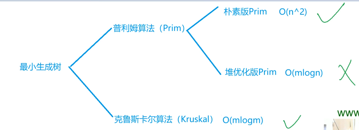
朴素版prim算法
算法思想
Prim算法每次循环都将一个蓝点u变为白点,并且次蓝点u与白点相连的最小边权min[u]还是当前所有蓝点中最小的。
这样相当于向生成树中添加了n-1次最小的边,最后得到的一定是最小生成树。
算法图解:
通过下图最小生成树的求解模拟来理解上面的思想。
蓝点和虚线代表未进入最小生成树的点、边;白点和实线代表已进入最小生成树的点、边。

此为原始的加权连通图。每条边一侧的数字代表其权值。

顶点D被任意选为起始点。顶点A、B、E和F通过单条边与D相连。A是距离D最近的顶点,因此将A及对应边AD以高亮表示。

下一个顶点为距离D或A最近的顶点。B距D为9,距A为7,E为15,F为6。因此,F距D或A最近,因此将顶点F与相应边DF以高亮表示。

算法继续重复上面的步骤。距离A为7的顶点B被高亮表示。

在当前情况下,可以在C、E与G间进行选择。C距B为8,E距B为7,G距F为11。E最近,因此将顶点E与相应边BE高亮表示。

这里,可供选择的顶点只有C和G。C距E为5,G距E为9,故选取C,并与边EC一同高亮表示

顶点G是唯一剩下的顶点,它距F为11,距E为9,E最近,故高亮表示G及相应边EG。

现在,所有顶点均已被选取,图中绿色部分即为连通图的最小生成树。在此例中,最小生成树的权值之和为39。
注意:
最短路dijkstra算法,每次取的是距源点最近的点。
Prim算法,每次取得是距已选点集合最近的点。
时间复杂度: \(O(n^2)\),可以用二叉堆优化到\(O(mlogn)\)。
但用二叉堆优化不如直接用Kruskal算法更加方便。因此,Prim主要用于稠密图,尤其是完全图的最小生成树的求解
例题 局域网
#include <bits/stdc++.h>
using namespace std;

/*
求出最小生成树,用总长度减去最小生成树即为答案
*/

const int inf = 0x7fffffff;
const int maxn = 110;

int n = 0, m = 0;
int a[maxn][maxn] = {};
int ans = 0;
int v[maxn] = {}, d[maxn] = {};

void prim(int x)
{
	for(int i=1; i<=n; i++) d[i] = a[x][i];
	v[x] = true;
	for(int i=2; i<=n; i++)
	{
		int t = inf, k = 0;
		for(int j=1; j<=n; j++)
		{
			if(!v[j] && t>d[j])
			{
				t = d[j];
				k = j;
			}
		}
		v[k] = 1;
		ans += d[k];
		for(int j=1; j<=n; j++)
		{
			if(!v[j] && d[j]>a[k][j]) d[j] = a[k][j];
		}
	}
}

int main()
{
	int x = 0, y = 0, z = 0;
	int tot = 0;

	scanf("%d%d", &n, &m);
	memset(a, 0x3f, sizeof(a));
	for(int i=1; i<=m; i++)
	{
		scanf("%d%d%d", &x, &y, &z);
		a[x][y] = a[y][x] = z;
		tot += z;
	}

	prim(1);
	printf("%d\n", tot-ans);

	return 0;
}
堆优化prim算法
写法复杂,基本用不到
Kruskal算法
算法思想
1、Kruskal算法是一种用来寻找最小生成树的算法,两种算法都是贪心思想的应用。Kruskal算法在图中存在相同权值的边时也有效。
2、Kruskal算法每次从剩下的边中选择一条不会产生环路的具有最小耗费的边加入已选择的边的集合中。注意到所选取的边若产生环路则不可能形成一棵生成树。
步骤:
Kruskal算法分e步,其中e是网络中边的数目。按耗费递增的顺序来考虑这e条边,每次考虑一条边。
当考虑某条边时,若将其加入到已选边的集合中会出现环路,则将其抛弃,否则,将它选入。
算法说明:
Kruskal算法会生成多个生成树(即森林),关键步骤在于:
1、对图中的边按权值排序
2、新加入边时判断是否会在树中构成回路
3、当新加入的边的两端点分属于两颗不同的树时,合并这两棵树
算法图解:

首先第一步,我们有一张图Graph,有若干点和边

将所有的边的长度排序,用排序的结果作为我们选择边的依据。这里再次体现了贪心算法的思想。资源排序,对局部最优的资源进行选择,排序完成后,我们率先选择了边AD。这样我们的图就变成了上图

在剩下的边中寻找。我们找到了CE。这里边的权重也是5

依次类推我们找到了6,7,7,即DF,AB,BE。

下面继续选择, BC或者EF尽管现在长度为8的边是最小的未选择的边。但是现在他们已经连通了(对于BC可以通过CE,EB来连接,类似的EF可以通过EB,BA,AD,DF来接连)。所以不需要选择他们。类似的BD也已经连通了(这里上图的连通线用红色表示了)。最后就剩下EG和FG了。当然我们选择了EG。最后成功的图就是上图
注意: Kruskal算法不需要建图,只需要把所有边存下来即可。
时间复杂度: \(O(mlogm)\)
例题 局域网
#include <bits/stdc++.h>
using namespace std;

const int maxn = 110;
const int maxm = maxn * maxn;

int n = 0, m = 0; //n表示点数,m表示边数
int fa[maxn] = {}, ans = 0, sum = 0;
struct node
{
	int x, y, z;
	bool operator < (const node &nd) const
	{
		return z < nd.z;
	}
}e[maxm];

int findset(int x)
{
	if(fa[x] != x) fa[x] = findset(fa[x]);
	return fa[x];
}

void Kruskal()
{
	int t = 0;
	//按边权从小到大排序
	sort(e+1, e+1+m);
	//并查集初始化
	for(int i=1; i<=n; i++) fa[i] = i;
	//求最小生成树
	for(int i=1; i<=m; i++)
	{
		int fx = findset(e[i].x);
		int fy = findset(e[i].y);
		if(fx == fy) continue;
		fa[fy] = fx;
		ans += e[i].z;

		t++;
		if(t == n-1) break;
	}
}

int main()
{
	scanf("%d%d", &n, &m);
	for(int i=1; i<=m; i++)
	{
		scanf("%d%d%d", &e[i].x, &e[i].y, &e[i].z);
		sum += e[i].z;
	}

	Kruskal();
	printf("%d", sum - ans);

	return 0;
}
拓扑排序
一些概念
定义: 在一个\(DAG\)(有向无环图)中,将图中的顶点以线性方式进行排序,使得对于任何的顶点\(u\)到\(v\)的有向边\((u,v)\),都可以有\(u\)在\(v\)的前面。
目标: 将所有节点排序,使得排在前面的节点不能依赖于排在后面的节点。
构造拓扑序列的步骤:
1、从图中选择一个入度为零的点
2、输出该顶点,从图中删除此顶点及所有的出边
3、重复上面两步,直到所有顶点都输出,拓扑排序完成。或者图中不存在入度为零的点,此时说明图是有环图,拓扑排序无法完成,陷入死锁。
时间复杂度: \(O(n+m)\),n表示点数,m表示边数
样例:
给定一个\(DAG\),求出其拓扑排序
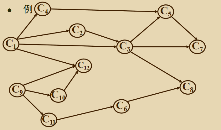
上图的拓扑序列可能是下面两种:
(C1, C2, C3, C4, C5, C7, C9, C10, C11, C6, C12, C8)
(C9, C10, C11, C6, C1, C12, C4, C2, C3, C5, C7, C8)
注意: 一个\(DAG\)的拓扑序列不唯一,与存图顺序有关,只要满足拓扑排序的定义即可
拓扑排序与\(bfs\):
1、\(bfs\)可用于有向图或无向图,有环或无环
2、拓扑排序只能把入度为\(0\)的点作为起点,\(bfs\)可以把任意点作为起点
3、因此拓扑排序可以认为是一种特殊的\(bfs\)
int in[maxn] = {};	//存储某个节点的入度

bool topsort()
{
	int cnt = 0;	//记录经过的节点数量
	queue<int> q;

	//将入度为0的节点入队
	for(int i=1; i<=n; i++)
	{
		if(in[i] == 0) q.push(i);
	}

	while(!q.empty())
	{
		int x = q.front();
		q.pop();
		cnt++;	//记录拓扑序列中点的个数

		for(int i=h[x]; i; i=nxt[i])
		{
			int y = to[i];
			in[y]--;
			if(in[y] == 0) q.push(y); 	//只有该点入度为0时,才入队
		}
	}
	if(cnt == n) return true;	//若拓扑序列中正好是n个点,说明所有点都已出现在拓扑序列中
	return false;	//否则说明图中有环
}
例题 家谱树
#include <bits/stdc++.h>
using namespace std;

/*
根据数据建图,然后跑一遍拓扑排序即可
*/

const int maxn = 110;
const int maxm = maxn*maxn;

int n = 0;
int head[maxn], to[maxm], nxt[maxm], tot = 0;
queue<int> q;
int v[maxn];
int in[maxn];

void addedge(int x, int y)
{
	nxt[++tot] = head[x];
	to[tot] = y;
	head[x] = tot;
}

void tpsort()
{
	for(int i=1; i<=n; i++)
	{
		if(in[i] == 0) q.push(i);
	}

	while(q.size())
	{
		int x = q.front();
		q.pop();
		printf("%d ", x);
		for(int i=head[x]; i; i=nxt[i])
		{
			int y = to[i];
			in[y]--;
			if(in[y] == 0) q.push(y);
		}
	}
}

int main()
{
	int x = 0;

	scanf("%d", &n);
	for(int i=1; i<=n; i++)
	{
		while(1)
		{
			scanf("%d", &x);
			if(x == 0) break;
			addedge(i, x);
			in[x]++;
		}
	}

	tpsort();

	return 0;
}
二分图

差分约束

判断是否合法
例题:提高题库 183.小K的农场
#include <bits/stdc++.h>
using namespace std;

const int maxn = 10010;
const int maxm = 30010;

int n = 0, m = 0;
int h[maxn] = {}, to[maxm] = {}, nxt[maxm] = {}, w[maxm] = {}, tot = 0;
bool vis[maxn] = {};
int dis[maxn] = {};

void addedge(int x, int y, int z)
{
	to[++tot] = y;
	w[tot] = z;
	nxt[tot] = h[x];
	h[x] = tot;
}

//dfs版spfa
void spfa(int x)
{
	vis[x] = true;
	for(int i=h[x]; i; i=nxt[i])
	{
		int y = to[i];
		if(dis[y] > dis[x] + w[i])
		{
			if(vis[y])
			{
				printf("No");
				exit(0);
			}
			dis[y] = dis[x] + w[i];
			spfa(y);
		}
	}
	vis[x] = false;
}

int main()
{
	int p = 0, a = 0, b = 0, c = 0;
	scanf("%d%d", &n, &m);
	for(int i=1; i<=m; i++)
	{
		scanf("%d", &p);
		if(p == 1)
		{
			scanf("%d%d%d", &a, &b, &c);
			addedge(a, b, -c);
		}
		else if(p == 2)
		{
			scanf("%d%d%d", &a, &b, &c);
			addedge(b, a, c);
		}
		else
		{
			scanf("%d%d", &a, &b);
			addedge(b, a, 0);
			addedge(a, b, 0);
		}
	}

	//建立超级源点
	for(int i=1; i<=n; i++) addedge(0, i, 0);

	//判断有无负环
	memset(dis, 0x3f, sizeof(dis));
	dis[0] = 0;
	spfa(0);
	printf("Yes");
}
求最小值
最近公共祖先(LCA)
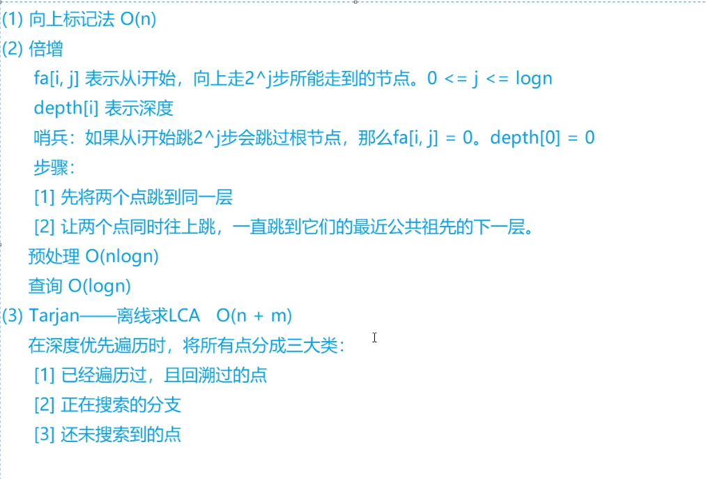
倍增法
倍增法为在线算法
例题:提高题库 315.Distance Queries 距离咨询
#include <bits/stdc++.h>
using namespace std;

const int maxn = 40010;
const int maxm = 80010;

int n = 0, m = 0, q = 0;
int h[maxn] = {}, nxt[maxm] = {}, to[maxm] = {}, w[maxm] = {}, tot = 0;
int f[maxn][30] = {}, dis[maxn] = {}, dep[maxn] = {};

void addedge(int x, int y, int z)
{
	to[++tot] = y;
	w[tot] = z;
	nxt[tot] = h[x];
	h[x] = tot;
}

//①该题中任意两个农场之间都有且只有一条路径
//所以可以指定任意一个点为根节点
//并且只要dfs的过程中更新路径,该路径即为两点间的距离
//②dfs的过程中可以顺便维护节点深度
void dfs(int x, int fa)
{
	dep[x] = dep[fa] + 1;
	f[x][0] = fa;

	for(int i=h[x]; i; i=nxt[i])
	{
		int y = to[i];
		if(y == fa) continue;
		dis[y] = dis[x] + w[i];

		dfs(y, x);
	}
}

//倍增法求lca
int lca(int x, int y)
{
	if(dep[x] < dep[y]) swap(x, y);

	//x和y跳到同一深度
	int d = dep[x] - dep[y];
	for(int i=0; i<30; i++)
	{
		if(d & (1<<i)) x = f[x][i];
	}

	if(x == y) return x;

	//x和y同时往上跳
	for(int i=29; i>=0; i--)
	{
		if(f[x][i] != f[y][i])
		{
			x = f[x][i];
			y = f[y][i];
		}
		if(f[x][0] == f[y][0]) break;
	}

	return f[x][0];
}

int main()
{
	int x = 0, y = 0, z = 0;
	char c;
	scanf("%d%d", &n, &m);
	for(int i=1; i<=m; i++)
	{
		scanf("%d%d%d %c", &x, &y, &z, &c);
		addedge(x, y, z);
		addedge(y, x, z);
	}

	dfs(1, 0);

	//ST表初始化
	for(int j=1; j<30; j++)
	{
		for(int i=1; i<=n; i++)
		{
			f[i][j] = f[f[i][j-1]][j-1];
		}
	}

	scanf("%d", &q);
	while(q--)
	{
		scanf("%d%d", &x, &y);

		int t = lca(x, y);
		printf("%d\n", dis[x] + dis[y] - 2 * dis[t]);
	}

	return 0;
}
tarjan算法求lca
简介: tarjan算法为离线算法,需要使用并查集记录某个节点的祖先节点
主要思路: 首先初始化每个节点的祖先节点为自身,任选一个节点进行\(dfs\),遍历完某个节点及其子节点后,将该点的父亲节点设置为该点的祖先节点,然后查询和这个点相关的所有询问,当另一端点\(v\)已经遍历过时,该端点\(v\)的祖先节点,即这两个点的最近公共祖先(\(lca\))。
具体实现:
1、保存查询信息时,注意双向,即\(u->\)和\(v->u\)都要保存
2、初始化并查集,将每个点的祖先设置为其自身
3、开始\(dfs\),遍历完每个节点即其子节点后,将该点的祖先节点设置为其父节点
4、遍历完某个点\(u\)的所有子节点后,开始查询与\(u\)点相关的询问,假设两个点为\((u, v)\),则可能出现以下情况
①\(v\)还没有遍历过。直接跳过,等待遍历到\(v\)时,再找\(u\)
②\(v\)为\(u\)的子节点。此时找\(v\)的祖先节点,祖先节点一定是\(u\),即他们的\(lca\)。
③\(v\)和\(u\)属于不同的子树。此时\(v\)和\(u\)一定处于一棵大的子树中,找\(v\)的祖先节点,就是该大子树的根节点,即他们的\(lca\)。
5、最后输出结果
时间复杂度: \(O(mα(m+n,n)+n)\),可近似认为是\(O(m+n)\)
例题: LG3379 【模板】最近公共祖先(LCA)
#include <bits/stdc++.h>
using namespace std;

const int maxn = 5e5 + 10;
const int maxm = 5e5 + 10;

int n = 0, m = 0, root = 0;
int h[maxn] = {}, to[maxn<<1] = {}, nxt[maxn<<1] = {}, tot = 0;
struct node
{
	int v, idx;			//指向的点和该询问的位置
};
vector<node> qry[maxn];	//存储查询信息
int fa[maxn] = {};		//并查集变量
int ans[maxm] = {};		//存储最终的答案
bool vis[maxn] = {};	//存储该节点是否已访问过

void addedge(int x, int y)
{
	to[++tot] = y;
	nxt[tot] = h[x];
	h[x] = tot;
}

//找x的祖先
int findset(int x)
{
	if(x == fa[x]) return fa[x];
	return fa[x] = findset(fa[x]);
}

//求lca
void dfs(int x)
{
	int y = 0;

	vis[x] = true;
	for(int i=h[x]; i; i=nxt[i])
	{
		y = to[i];
		if(vis[y]) continue;

		dfs(y);
		fa[y] = x;
	}

	for(auto nd : qry[x])
	{
		if(vis[nd.v])
		{
			ans[nd.idx] = findset(nd.v);
		}
	}
}

int main()
{
	int x = 0, y = 0;

	scanf("%d%d%d", &n, &m, &root);
	for(int i=1; i<n; i++)
	{
		scanf("%d%d", &x, &y);
		addedge(x, y);
		addedge(y, x);
	}
	for(int i=1; i<=m; i++)
	{
		scanf("%d%d", &x, &y);
		qry[x].push_back({y, i});
		qry[y].push_back({x, i});
	}

	for(int i=1; i<=n; i++) fa[i] = i;
	dfs(root);
	for(int i=1; i<=m; i++) printf("%d\n", ans[i]);

	return 0;
}
Tarjan
一些概念
无向连通图的搜索树:在无向连通图中任选一个节点出发进行深度优先遍历,每个点只访问一次。所有发生递归的边\((x,y)\)(换言之,从\(x\)到\(y\)是对\(y\)的第一次访问)构成一棵树,我们把他称为"无向连通图的搜索树"。
时间戳:在图的深度优先遍历过程中,按照每个节点第一次被访问的时间顺序,依次给予\(N\)个节点\(1\)~\(N\)的整数标记,该标记被称为“时间戳”,记为\(dfn[x]\)
追溯值: 设\(subtree(x)\)表示搜索树中以\(x\)为根的子树。\(low[x]\)定义为以下节点的时间戳的最小值
1、\(subtree(x)\)中的节点
2、通过1条不在搜索树上的边,能够到达\(subtree(x)\)的节点。
计算追溯值:
先令\(low[x]=dfn[x]\),然后考虑从\(x\)出发的每条边\((x, y)\)
1、树边,若在搜索树上\(x\)是\(y\)的父节点,则令\(low[x]=min(low[x],low[y])\)
2、非树边,若无向边\((x, y)\)不是搜索树上的边,则令\(low[x]=min(low[x],dfn[y])\)
割边
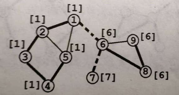
割边或桥:对于无向图 \(G=(V, E)\),若对于\(e∈E\),从图中删去边\(e\)之后,\(G\)分裂成两个不相连的子图,则称\(e\)为\(G\)的割边或桥。
ps:树中所有边都是桥
概念:无向边\((x, y)\)是桥,当且仅当搜索树上存在\(x\)的一个子节点\(y\),满足\(dfn[x]<low[y]\),即追溯不到更小的点
ps:桥一定是搜索树中的边,并且一个简单环中的边一定都不是桥

上图有两条割边,1->6和6->7
割边算法模板
#include <bits/stdc++.h>
using namespace std;

const int maxn = 100010;
const int maxm = 1000010;

int n = 0, m = 0;
//存图
int h[maxn] = {}, to[maxm] = {}, nxt[maxm] = {}, tot = 0;
//dfn:时间戳   low:追溯值
int dfn[maxn] = {}, low[maxn] = {}, num = 0;
bool bridge[maxm] = {};

void addedge(int x, int y)
{
	to[++tot] = y;
	nxt[tot] = h[x];
	h[x] = tot;
}

void tarjan(int x, int in_edge)
{
	dfn[x] = low[x] = ++num;
	for(int i=h[x]; i; i=nxt[i])
	{
		int y = to[i];
		if(!dfn[y])	//树边
		{
			tarjan(y, i);
			low[x] = min(low[x], low[y]);

			//此时已经遍历完x的子节点,又回溯到了x
			if(dfn[x] < low[y]) //说明经过(x,y)边,无法到达比x更早的点
			{
				//i和i^1是同一条边
				bridge[i] = bridge[i^1] = true;
			}
		}
		//i == (in_edge ^ 1)表示与i是同一条边
		//i != (in_edge ^ 1)说明是非树边
		else if(i != (in_edge ^ 1))
		{
			low[x] = min(low[x], dfn[y]);
		}
	}
}

int main()
{
	int x = 0, y = 0;

	//这里是为了保证i和i^1是同一条边
	//这样边的编号从2开始,2/3为一对,4/5为一对,以此类推
	tot = 1;
	scanf("%d%d", &n, &m);
	for(int i=1; i<=m; i++)
	{
		scanf("%d%d", &x, &y);
		addedge(x, y);
		addedge(y, x);
	}
	for(int i=1; i<=n; i++)
	{
		if(!dfn[i]) tarjan(i, 0);
	}
	for(int i=2; i<tot; i++)
	{
		if(bridge[i])
		{
			printf("%d %d\n", to[i^1], to[i]);
		}
	}

	return 0;
}
割点
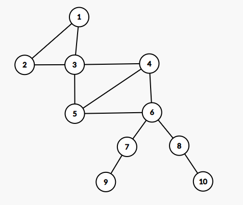
割点:对于无向图 \(G=(V, E)\),若对于\(x∈V\),从图中删去节点\(x\)以及所有与\(x\)关联的边之后,\(G\)分裂成两个或两个以上不相连的子图,则称\(x\)为\(G\)的割点。
ps:树中度为1的点(叶子结点)都不是割点,其他都是割点
条件:若\(x\)不是搜索树的根节点(深度优先遍历的起点),则\(x\)是割点当且仅当搜索树上存在\(x\)的一个子节点\(y\),满足:\(dfn[x]<=low[y]\)
特点:
1、若\(x\)是搜索树的根节点,则\(x\)是割点当且仅当搜索树上存在至少两个子节点\(y1,y2\)满足上述条件。
2、下面非空,即不能是叶子节点
3、上下只能通过\(x\)相通,即y子树不能追溯到比x更早的点
下图中共有两个割点,分别是时间戳为1和6的两个点
割点算法模板
#include <bits/stdc++.h>
using namespace std;

const int maxn = 100010;
const int maxm = 1000010;

int n = 0, m = 0;
//存图
int h[maxn] = {}, to[maxm] = {}, nxt[maxm] = {}, tot = 0;
//dfn:时间戳   low:追溯值
int dfn[maxn] = {}, low[maxn] = {}, num = 0;
int root = 0;
bool cut[maxn] = {};
int cnt = 0;

void addedge(int x, int y)
{
	to[++tot] = y;
	nxt[tot] = h[x];
	h[x] = tot;
}

void tarjan(int x)
{
	dfn[x] = low[x] = ++num;
	int flag = 0;	//记录x有多少个不能回溯到x之前的子节点
	for(int i=h[x]; i; i=nxt[i])
	{
		int y = to[i];
		if(!dfn[y])	//树边
		{
			tarjan(y);
			low[x] = min(low[x], low[y]);

			//此时已经遍历完x的子节点,又回溯到了x
			if(dfn[x] <= low[y]) //y无法到达比x更早的点
			{
				flag++;
				if(x != root || flag > 1)
				{
					//如果统计割点数量,这里要判断一下是否已标记
					//因为一个割点可能会被重复访问
					//下图中点6就会被访问两次
					if(!cut[x])
					{
						cut[x] = true;
						cnt++;
					}
				}
			}
		}
		else
		{
			low[x] = min(low[x], dfn[y]);
		}
	}
}

int main()
{
	int x = 0, y = 0;

	scanf("%d%d", &n, &m);
	for(int i=1; i<=m; i++)
	{
		scanf("%d%d", &x, &y);
		if(x == y) continue;
		addedge(x, y);
		addedge(y, x);
	}
	for(int i=1; i<=n; i++)
	{
		if(!dfn[i])
		{
			root = i;	//方便后面判断是否为根节点
			tarjan(i);
		}
	}
	for(int i=1; i<=n; i++)
	{
		if(cut[i]) printf("%d ", i);
	}
	printf("are cut-vertexes");

	return 0;
}
无向图的双连通分量
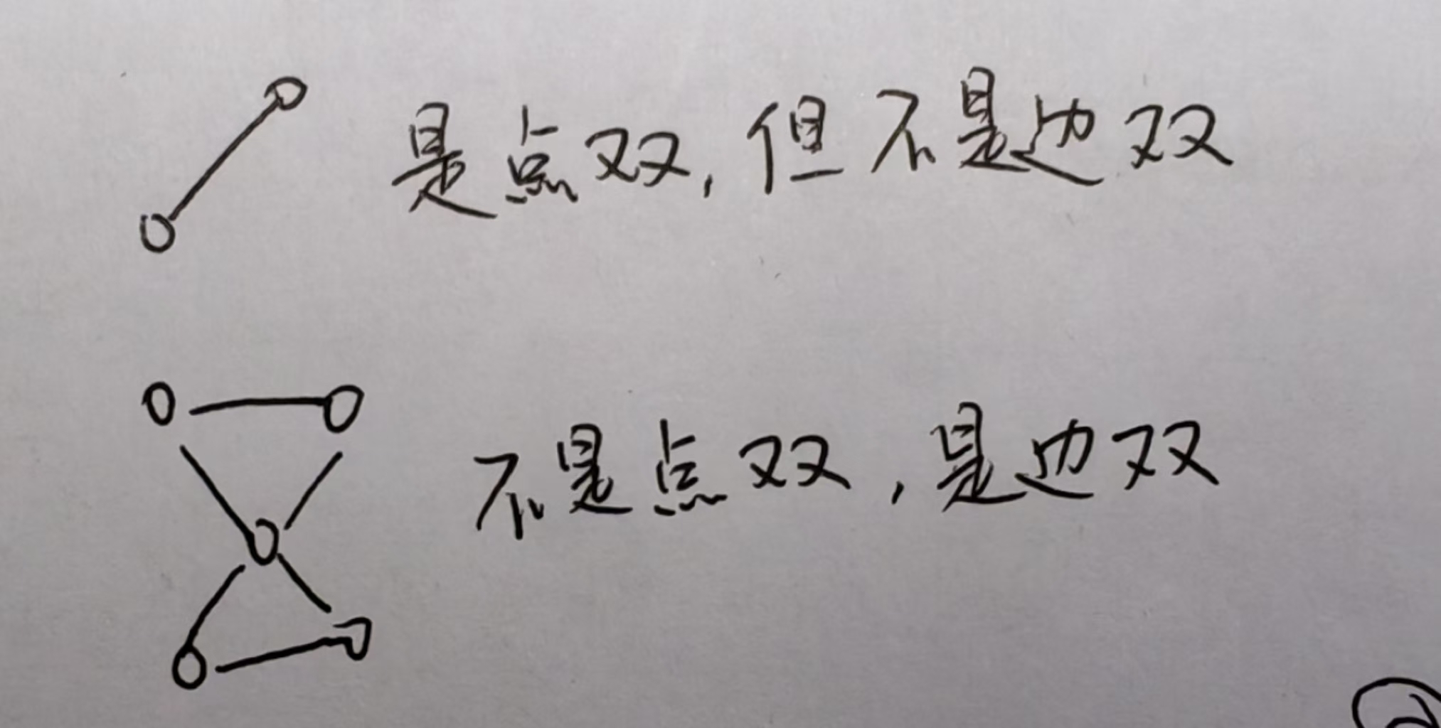
点双连通图:若一张无向连通图不存在割点,则称它为“点双连通图”
边双连通图:若一张无向连通图不存在桥,则称他为“边双连通图”
点双连通分量:无向图的极大点双连通子图被称为“点双连通分量”\(v-DCC\)
边双连通分量:无向连通图的极大边双连通子图被称为“边双连通分量”简称\(e-DCC\)
一张无向连通图是“点双连通图”,当且仅当满足下列两个条件之一:
1、图的顶点数不超过2。(ps:意思是当一个图仅有1个或2个顶点时,一定是点双)
2、图中任意两点都同时包含在至少一个简单环中。(ps:“简单环”指的是不自交的环,也就是我们通常画出的环)
边双连通分量(e-DCC)的求法模板:
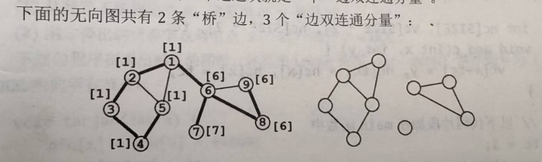
算法:先用\(Tarjan\)算法标记出所有的桥边。然后,再对整个无向图执行一次深度优先遍历(遍历的过程中不访问桥边),划分出每个连通块。
下面的代码在\(Tarjan\)求桥的基础上,计算出数组\(c\),\(c[x]\)表示节点\(x\)所属的“边双连通分量”的编号
#include <bits/stdc++.h>
using namespace std;

const int maxn = 100010;
const int maxm = 1000010;

int n = 0, m = 0;
//存图
int h[maxn] = {}, to[maxm] = {}, nxt[maxm] = {}, tot = 0;
//dfn:时间戳   low:追溯值
int dfn[maxn] = {}, low[maxn] = {}, num = 0;
bool bridge[maxm] = {};
int c[maxn] = {}, dcc = 0;

void addedge(int x, int y)
{
	to[++tot] = y;
	nxt[tot] = h[x];
	h[x] = tot;
}

void tarjan(int x, int in_edge)
{
	dfn[x] = low[x] = ++num;
	for(int i=h[x]; i; i=nxt[i])
	{
		int y = to[i];
		if(!dfn[y])	//树边
		{
			tarjan(y, i);
			low[x] = min(low[x], low[y]);

			//此时已经遍历完y节点
			if(dfn[x] < low[y]) //说明经过(x,y)边,无法到达比x更早的点
			{
				//i和i^1是同一条边
				bridge[i] = bridge[i^1] = true;
			}
		}
		//i == (in_edge ^ 1)表示与i是同一条边
		//i != (in_edge ^ 1)说明是非树边
		else if(i != (in_edge ^ 1))
		{
			low[x] = min(low[x], dfn[y]);
		}
	}
}

void dfs(int x)
{
	c[x] = dcc;
	for(int i=h[x]; i; i=nxt[i])
	{
		int y = to[i];
		if(c[y] || bridge[i]) continue;
		dfs(y);
	}
}

int main()
{
	int x = 0, y = 0;

	//这里是为了保证i和i^1是同一条边
	//这样边的编号从2开始,2/3为一对,4/5为一对,以此类推
	tot = 1;
	scanf("%d%d", &n, &m);
	for(int i=1; i<=m; i++)
	{
		scanf("%d%d", &x, &y);
		addedge(x, y);
		addedge(y, x);
	}
	for(int i=1; i<=n; i++)
	{
		if(!dfn[i]) tarjan(i, 0);
	}

	for(int i=1; i<=n; i++)
	{
		if(!c[i])
		{
			++dcc;
			dfs(i);
		}
	}
	printf("There are %d e-DCCs.\n", dcc);
	for(int i=1; i<=n; i++)
	{
		printf("%d belongs to DCC %d.\n", i, c[i]);
	}

	return 0;
}
e-DCC的缩点模板:
把每个\(e-DCC\)看做一个节点,把桥边\((x, y)\)看做连接编号为\(c[x]\)和\(c[y]\)的\(e-DCC\)对应节点的无向边,会产生一棵树(若原来的无向图不连通,则产生森林)。这种把\(e-DCC\)收缩为一个节点的方法就称为“缩点”。
下面的代码在\(Tarjan\)求桥、求\(e-DCC\)的参考程序基础上,把\(e-DCC\)缩点,构成一棵新的树(或森林),存储在另一个邻接表中
#include <bits/stdc++.h>
using namespace std;

const int maxn = 100010;
const int maxm = 1000010;

int n = 0, m = 0;
//存原图
int h[maxn] = {}, to[maxm] = {}, nxt[maxm] = {}, tot = 0;
//dfn:时间戳   low:追溯值
int dfn[maxn] = {}, low[maxn] = {}, num = 0;
bool bridge[maxm] = {};
int c[maxn] = {}, dcc = 0;
//存缩点后的图
int hc[maxn] = {}, toc[maxm] = {}, nxtc[maxn] = {}, totc = 0;

void addedge(int x, int y)
{
	to[++tot] = y;
	nxt[tot] = h[x];
	h[x] = tot;
}

void addedge_c(int x, int y)
{
	toc[++totc] = y;
	nxtc[totc] = hc[x];
	hc[x] = totc;
}

void tarjan(int x, int in_edge)
{
	dfn[x] = low[x] = ++num;
	for(int i=h[x]; i; i=nxt[i])
	{
		int y = to[i];
		if(!dfn[y])	//树边
		{
			tarjan(y, i);
			low[x] = min(low[x], low[y]);

			//此时已经遍历完y节点
			if(dfn[x] < low[y]) //说明经过(x,y)边,无法到达比x更早的点
			{
				//i和i^1是同一条边
				bridge[i] = bridge[i^1] = true;
			}
		}
		//i == (in_edge ^ 1)表示与i是同一条边
		//i != (in_edge ^ 1)说明是非树边
		else if(i != (in_edge ^ 1))
		{
			low[x] = min(low[x], dfn[y]);
		}
	}
}

void dfs(int x)
{
	c[x] = dcc;
	for(int i=h[x]; i; i=nxt[i])
	{
		int y = to[i];
		if(c[y] || bridge[i]) continue;
		dfs(y);
	}
}

int main()
{
	int x = 0, y = 0;

	//这里是为了保证i和i^1是同一条边
	//这样边的编号从2开始,2/3为一对,4/5为一对,以此类推
	tot = 1;
	scanf("%d%d", &n, &m);
	for(int i=1; i<=m; i++)
	{
		scanf("%d%d", &x, &y);
		addedge(x, y);
		addedge(y, x);
	}
	for(int i=1; i<=n; i++)
	{
		if(!dfn[i]) tarjan(i, 0);
	}

	for(int i=1; i<=n; i++)
	{
		if(!c[i])
		{
			++dcc;
			dfs(i);
		}
	}

	printf("There are %d e-DCCs.\n", dcc);
	for(int i=1; i<=n; i++)
	{
		printf("%d belongs to DCC %d.\n", i, c[i]);
	}

	totc = 1;
	for(int i=2; i<=tot; i++)
	{
		//第i条边为x->y,第i^1条边为y->x
		int x = to[i^1], y = to[i];
		if(c[x] == c[y]) continue;
		addedge_c(c[x], c[y]);
	}

	printf("缩点之后的森林,点数%d,边数%d\n", dcc, totc / 2);
	for(int i=2; i<totc; i+=2)
	{
		printf("%d %d\n", toc[i^1], toc[i]);
	}

	return 0;
}
点双连通分量(v-DCC)的求法模板:
定义:
1、若某个节点为孤立点,则它自己单独构成一个\(v-DCC\)。
2、除了孤立点外,点双连通分量的大小至少为2.
3、根据\(v-DCC\)定义中的“极大”性,虽然桥不属于任何\(e-DCC\),但是割点可能属于多个\(v-DCC\)。
下面的无向图共有2个割点,4个“点双连通分量”
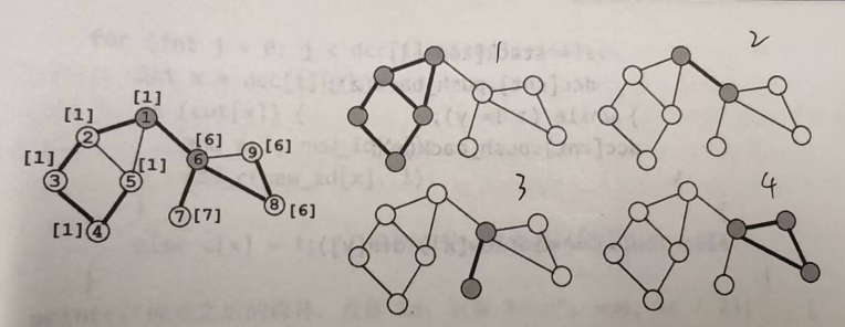
算法简介:
1、当一个节点第一次被访问时,把该节点入栈
2、当割点判定法则中的条件\(dfn[x]<=low[y]\)成立时,无论x是否为根,都要
(1)从栈顶不断弹出节点,直至节点y被弹出
(2)刚才弹出的所有节点与节点\(x\)一起构成一个\(v-DCC\)。
下面的程序在求割点的同时,计算出\(vector\)数组\(dcc\),\(dcc[i]\)保存编号为\(i\)的\(v-DCC\)中的所有节点
#include <bits/stdc++.h>
using namespace std;

const int maxn = 100010;
const int maxm = 1000010;

int n = 0, m = 0;
//存图
int h[maxn] = {}, to[maxm] = {}, nxt[maxm] = {}, tot = 0;
//dfn:时间戳   low:追溯值
int dfn[maxn] = {}, low[maxn] = {}, num = 0;
int root = 0;
bool cut[maxn] = {};	//cut[x]表示x是否为割点
//cnt表示点双的数量
int stk[maxn] = {}, top = 0, cnt = 0;
vector<int> dcc[maxn];	//dcc[x]表示第x个点双中包含的节点

void addedge(int x, int y)
{
	to[++tot] = y;
	nxt[tot] = h[x];
	h[x] = tot;
}

void tarjan(int x)
{
	dfn[x] = low[x] = ++num;
	int flag = 0;	//记录x有多少个不能回溯到x之前的子节点
	stk[++top] = x;

	if(x == root && h[x] == 0)	//孤立点
	{
		dcc[++cnt].push_back(x);
		return;
	}

	for(int i=h[x]; i; i=nxt[i])
	{
		int y = to[i];
		if(!dfn[y])	//树边
		{
			tarjan(y);
			low[x] = min(low[x], low[y]);

			//此时已经遍历完x的子节点,又回溯到了x
			if(dfn[x] <= low[y]) //y无法到达比x更早的点
			{
				flag++;
				if(x != root || flag > 1) cut[x] = true;
				cnt++;
				int z = 0;
				do
				{
					z = stk[top--];
					dcc[cnt].push_back(z);
				}while(z != y);
				dcc[cnt].push_back(x);
			}
		}
		else
		{
			low[x] = min(low[x], dfn[y]);
		}
	}
}

int main()
{
	int x = 0, y = 0;

	scanf("%d%d", &n, &m);
	for(int i=1; i<=m; i++)
	{
		scanf("%d%d", &x, &y);
		if(x == y) continue;
		addedge(x, y);
		addedge(y, x);
	}
	for(int i=1; i<=n; i++)
	{
		if(!dfn[i])
		{
			root = i;	//方便后面判断是否为根节点
			tarjan(i);
		}
	}
	for(int i=1; i<=n; i++)
	{
		if(cut[i]) printf("%d ", i);
	}
	printf("are cut-vertexes");

	for(int i=1; i<=cnt; i++)
	{
		printf("v-DCC #%d:", i);
		for(int j=0; j<dcc[i].size(); j++)
		{
			printf(" %d", dcc[i][j]);
		}
		printf("\n");
	}

	return 0;
}
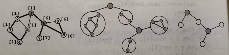
v-DCC的缩点模板:
v-DCC的缩点比e-DCC要复杂一些——因为一个割点可能属于多个v-DCC。
设图中共有p个割点和t个v-DCC。我们建立一张包含p+t个节点的新图,把每个v-DCC和每个割点都作为新图中的节点,并在每个割点与包含它的所有v-DCC之间连边。
容易发现,这张新图其实是一棵树(或森林),如下图所示:
#include <bits/stdc++.h>
using namespace std;

const int maxn = 100010;
const int maxm = 1000010;

int n = 0, m = 0;
//存图
int h[maxn] = {}, to[maxm] = {}, nxt[maxm] = {}, tot = 0;
//dfn:时间戳   low:追溯值
int dfn[maxn] = {}, low[maxn] = {}, num = 0;
int root = 0;
bool cut[maxn] = {}, c[maxn] = {};	//cut[x]表示x是否为割点,c[x]表示x属于哪个v-DCC
//cnt表示点双的数量
int stk[maxn] = {}, top = 0, cnt = 0;
vector<int> dcc[maxn];	//dcc[x]表示第x个点双中包含的节点
int new_id[maxn] = {};	//new_id[x]表示割点x的新编号
int hc[maxn] = {}, toc[maxm] = {}, nxtc[maxm] = {}, totc = 0;

void addedge(int x, int y)
{
	to[++tot] = y;
	nxt[tot] = h[x];
	h[x] = tot;
}

void addedge_c(int x, int y)
{
	toc[++totc] = y;
	nxtc[totc] = h[x];
	hc[x] = totc;
}

void tarjan(int x)
{
	dfn[x] = low[x] = ++num;
	int flag = 0;	//记录x有多少个不能回溯到x之前的子节点
	stk[++top] = x;

	if(x == root && h[x] == 0)	//孤立点
	{
		dcc[++cnt].push_back(x);
		return;
	}

	for(int i=h[x]; i; i=nxt[i])
	{
		int y = to[i];
		if(!dfn[y])	//树边
		{
			tarjan(y);
			low[x] = min(low[x], low[y]);

			//此时已经遍历完x的子节点,又回溯到了x
			if(dfn[x] <= low[y]) //y无法到达比x更早的点
			{
				flag++;
				if(x != root || flag > 1) cut[x] = true;
				cnt++;
				int z = 0;
				do
				{
					z = stk[top--];
					dcc[cnt].push_back(z);
				}while(z != y);
				dcc[cnt].push_back(x);
			}
		}
		else
		{
			low[x] = min(low[x], dfn[y]);
		}
	}
}

int main()
{
	int x = 0, y = 0;

	scanf("%d%d", &n, &m);
	for(int i=1; i<=m; i++)
	{
		scanf("%d%d", &x, &y);
		if(x == y) continue;
		addedge(x, y);
		addedge(y, x);
	}
	for(int i=1; i<=n; i++)
	{
		if(!dfn[i])
		{
			root = i;	//方便后面判断是否为根节点
			tarjan(i);
		}
	}
	for(int i=1; i<=n; i++)
	{
		if(cut[i]) printf("%d ", i);
	}
	printf("are cut-vertexes");

	for(int i=1; i<=cnt; i++)
	{
		printf("v-DCC #%d:", i);
		for(int j=0; j<dcc[i].size(); j++)
		{
			printf(" %d", dcc[i][j]);
		}
		printf("\n");
	}

	//给每个割点一个新的编号(编号从cnt+1开始)
	num = cnt;
	for(int i=1; i<=n; i++)
	{
		if(cut[i]) new_id[i] = ++num;
	}
	//建新图,从每个v-DCC到它包含的所有割点连边
	totc = 1;
	for(int i=1; i<=cnt; i++)
	{
		for(int j=0; j<dcc[i].size(); j++)
		{
			int x = dcc[i][j];
			if(cut[x])
			{
				addedge_c(i, new_id[x]);	//i就是该v-DCC的编号,连线
				addedge_c(new_id[x], i);
			}
			else c[x] = i;
		}
	}

	printf("缩点之后的森林,点数%d,边数%d\n", num, totc / 2);
	printf("编号1~%d的为原图的v-DCC,编号>%d的为原图割点\n", cnt, cnt);
	for(int i=2; i<totc; i+=2)
	{
		printf("%d %d\n", toc[i^1], toc[i]);
	}

	return 0;
}
有向图连通性
流图:给定有向图\(G=(V, E)\),若存在\(r∈V\),满足从\(r\)出发能够到达V中所有的点,则称\(G\)是一个“流图”,记为\((G, r)\),其中\(r\)称为流图的源点
流图\((G, r)\)的搜索树:在一个流图\((G, r)\)上从\(r\)出发进行深度优先遍历,每个点只访问一次。所有发生递归的边\((x, y)\)(换言之,从\(x\)到\(y\)是对\(y\)的第一次访问)构成一棵以\(r\)为根的数,我们把他称为流图\((G, r)\)的搜索树
时间戳: 在深度优先遍历的过程中,按照每个节点第一次被访问的时间顺序,一次给予流图中的\(N\)个节点1~\(N\)的整数标记,该标记被称为时间戳,记为\(dfn[x]\)
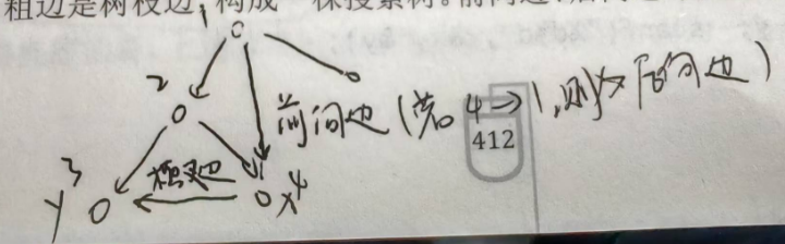
流图中的每条有向边\((x, y)\)必然是以下四种之一:
1、树枝边:指搜索树中的边,即\(x\)是\(y\)的父节点
2、前向边:指搜索树中\(x\)是\(y\)的祖先节点(没啥用,因为搜索树上本来就存在\(x\)到\(y\)的路径)
3、后向边:指搜索树中\(y\)是\(x\)的祖先节点(非常有用,因为它可以和搜索树上从\(y\)到\(x\)的路径一起构成环)
4、横叉边:指除了以上三种情况之外的边,他一定满足\(dfn[y]<dfn[x]\)(视情况而定,如果从\(y\)出发能找到一条路径回到\(x\)的祖先节点,那么\((x, y)\)就是有用的)
强连通图:给定一张有向图,若对于图中任意两个节点\(x,y\),既存在从\(x\)到\(y\)的路径,也存在从\(y\)到\(x\)的路径,则称该有向图是“强连通图”
强联通分量:有向图的极大强联通子图被称为“强联通分量”,简称“SCC”
追溯值: 设\(subtree(x)\)表示流图的搜索树中以\(x\)为根的子树。\(x\)的追溯值\(low[x]\)定义为满足以下条件的节点的最小时间戳:
1、该点在栈中(即遍历过该点)
2、存在一条从\(subtree(x)\)出发的有向边,以该点为终点(即存在横向边或后向边能到达该点)
追溯值的计算:
1、当节点\(x\)第一次被访问时,把\(x\)入栈,初始化\(low[x]=dfn[x]\)
2、扫描从\(x\)出发的每条边\((x, y)\)
(1)若\(y\)没被访问过,则说明\((x, y)\)是树枝边,递归访问\(y\),从\(y\)回溯之后,令\(low[x]=min(low[x], low[y])\)
(2)若\(y\)被访问过并且\(y\)在栈中,则说明\((x, y)\)是后向边,则令\(low[x]=min(low[x], dfn[y])\)
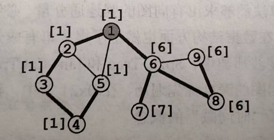
求强连通分量: 从\(x\)回溯之前,判断是否有\(low[x]=dfn[x]\)(说明\(subtree(x)\)追溯不到更高点了,此时出栈,则在最高点时出栈)。若成立,则不断从栈中弹出节点,直至\(x\)出栈。
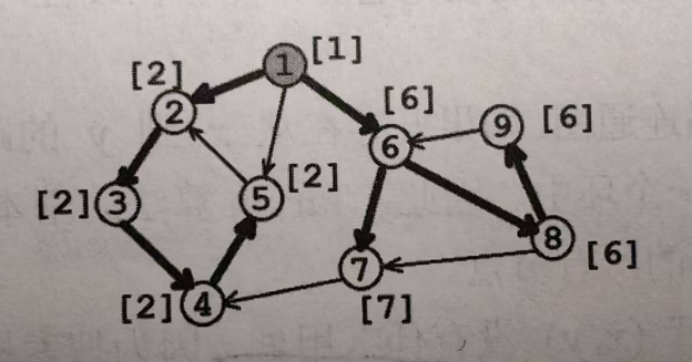
上图共有4个强联通分量(scc),分别是(2,3,4,5)(7)(6,8,9)(1)
强联通分量判定法则:
若从\(x\)回溯前,有\(low[x]=dfn[x]\)成立,则栈中从\(x\)到栈顶的所有节点构成一个强联通分量
scc算法模板:
下面的程序实现了\(Tarjan\)算法,求出数组\(c\),其中\(c[x]\)表示\(x\)所在的强连通分量的编号。另外,它还求出了\(vector\)数组\(scc\),\(scc[i]\)记录了编号为\(i\)的强连通分量中的所有节点。整张图同有\(cnt\)个强连通分量
#include <bits/stdc++.h>
using namespace std;

const int maxn = 100010;
const int maxm = 1000010;

int n = 0, m = 0;
//存图
int h[maxn] = {}, to[maxm] = {}, nxt[maxm] = {}, tot = 0;
//dfn:时间戳   low:追溯值
int dfn[maxn] = {}, low[maxn] = {}, num = 0;
//stk:数组表示栈
//ins[x]:表示x是否在栈中
//c[x]:表示x属于哪个scc
int stk[maxn] = {}, top = 0, ins[maxn] = {}, c[maxn] = {}, cnt = 0;
//scc[x]:表示第x个scc中的点
vector<int>scc[maxn] = {};

void addedge(int x, int y)
{
	to[++tot] = y;
	nxt[tot] = h[x];
	h[x] = tot;
}

void tarjan(int x)
{
	int y = 0;
	dfn[x] = low[x] = ++num;	//初始是时间戳等于追溯值
	stk[++top] = x;
	ins[x] = 1;

	for(int i=h[x]; i; i=nxt[i])
	{
		y = to[i];
		if(!dfn[y])
		{
			tarjan(y);
			//树枝边,回溯是更新low[x]
			low[x] = min(low[x], low[y]);
		}
		else if(ins[y])	//在栈中,即表示之前访问过
		{
			//横向边或后向边
			low[x] = min(low[x], dfn[y]);
		}
	}

	if(dfn[x] == low[x])
	{
		cnt++;
		do
		{
			y = stk[top--];	//出栈
			ins[y] = 0;
			c[y] = cnt;	//标记该点属于哪个scc
			scc[cnt].push_back(y);	//将该点加入对应scc的容器
		}while(x != y);
	}
}

int main()
{
	int x = 0, y = 0;

	scanf("%d%d", &n, &m);
	for(int i=1; i<=m; i++)
	{
		scanf("%d%d", &x, &y);
		addedge(x, y);
	}
	for(int i=1; i<=n; i++)
	{
		if(!dfn[i]) tarjan(i);
	}

	return 0;
}
scc缩点模板:
#include <bits/stdc++.h>
using namespace std;

/*
1、求出该图中的强联通分量scc
2、将scc进行缩点后,形成一个新图
*/

const int maxn = 500010;
const int maxm = 500010;

int n = 0, m = 0;
int h[maxn] = {}, to[maxm] = {}, nxt[maxm] = {}, tot = 0;
int dfn[maxn] = {}, low[maxn] = {}, num = 0;
int stk[maxn] = {}, top = 0, ins[maxn] = {}, cnt = 0, c[maxn] = {};
vector<int> scc[maxn] = {};
int hc[maxn] = {}, toc[maxm] = {}, nxtc[maxm] = {}, totc = 0;

void addedge(int x, int y)
{
	to[++tot] = y;
	nxt[tot] = h[x];
	h[x] = tot;
}

void addedge_c(int x, int y)
{
	toc[++totc] = y;
	nxtc[totc] = hc[x];
	hc[x] = totc;
}

void tarjan(int x)
{
	int y = 0;
	dfn[x] = low[x] = ++num;
	stk[++top] = x;
	ins[x] = 1;

	for(int i=h[x]; i; i=nxt[i])
	{
		y = to[i];
		if(!dfn[y])
		{
			tarjan(y);

			low[x] = min(low[x], low[y]);
		}
		else if(ins[y])
		{
			low[x] = min(low[x], dfn[y]);
		}
	}

	if(dfn[x] == low[x])
	{
		cnt++;
		do
		{
			y = stk[top--];
			ins[y] = 0;
			c[y] = cnt;
			scc[cnt].push_back(y);
		}while(x != y);
	}
}

int main()
{
	int x = 0, y = 0;

	scanf("%d%d", &n, &m);
	for(int i=1; i<=m; i++)
	{
		scanf("%d%d", &x, &y);
		addedge(x, y);
	}

	//tarjan求scc模板
	for(int i=1; i<=n; i++)
	{
		if(!dfn[i]) tarjan(i);
	}

	//缩点,建新图
	for(int x=1; x<=n; x++)
	{
		for(int i=h[x]; i; i=nxt[i])
		{
			y = to[i];
			if(c[x] == c[y]) continue;
			addedge_c(c[x], c[y]);
		}
	}

	return 0;
}
树链剖分
重链剖分
概念
树链剖分用于将树分割成若干条链的形式,以维护树上路径的信息。
具体来说,将整棵树剖分为若干条链,使它们组合成线性结构,然后用其他数据结构(如线段树、树状数组、分块)维护信息。
一些定义
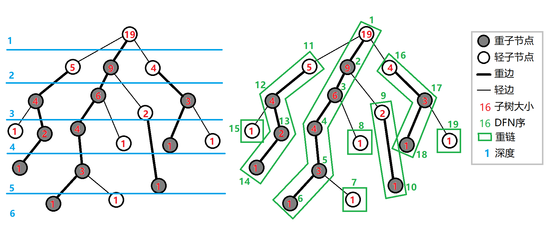
重子节点:表示其子节点中子树最大的子节点。如果有多个子树最大的子节点,取其一。如果没有子节点,就无重子节点
轻子节点:表示剩余的所有子节点
重边:从该节点到其重子节点的边为重边
轻边:从该节点到其轻子节点的边为轻边
重链:若干条首尾衔接的重边构成重链
把落单的节点也当作重链,那么整棵树就被剖分成若干条重链
一些性质
1、当树的节点为\(n\)时,最多有\(n-1\)条重链(特殊的,当树只有1个节点时,只有1条重链)
2、树上每个节点都属于且仅属于一条重链
3、重链开头的节点只能是根节点或轻子节点
4、所有的重链将整棵树完全剖分
5、在剖分时,重边优先遍历,最后树的\(dfs\)序上,重链内的\(dfs\)序是连续的。按\(dfn\)排序后的序列即为剖分后的链。
6、一棵子树内的\(dfs\)序是连续的
7、当向下经过一条轻边时,所在子树的大小至少会除以2
8、对于树上的任意一条路径,都可以被拆分成不超过\(O(logn)\)条重链。
解释上面的性质:
1、每条重链的末尾都是叶子节点,而叶子节点又只能属于一条重链,因此重链的条数等于叶子的数量,当树为星型结构时,重链最多,为\(n-1\)条
7、轻边\((u,v)\),\(size(v)<=size(u)/2\)
8、每增加一条重链,必定是通过轻边跳过去,所以重链的数量等于轻边的数量,而每经过一条轻边,点的数量至少会减少一半,所以最多经过\(logn\)条轻边,重链的数量最多也是\(logn\)。假如求\(x->y\)经过的重链条数,不用管\(lca\),直接\(x\)当成根节点思考就可以。
应用
1、求lca
2、拆分成链,用数据结构维护
具体实现
- \(fa(x)\)表示节点\(x\)在树上的父亲
- \(dep(x)\)表示节点\(x\)在树上的深度
- \(siz(x)\)表示节点\(x\)的子树的节点个数
- \(son(x)\)表示节点\(x\)的重儿子
- \(top(x)\)表示节点\(x\)所在重链的顶部节点(深度最小)
- \(dfn(x)\)表示节点\(x\)的\(dfs\)序,也是其在线段树中的编号
- \(rnk(x)\)表示\(dfs\)序所对应的节点编号,有\(rnk(dfn(x))=x\)
我们进行两遍\(dfs\)预处理出这些值
第一次\(dfs\)求出\(fa(x)\),\(dep(x)\),\(siz(x)\),\(son(x)\)
第二次\(dfs\)求出\(top(x)\),\(dfn(x)\),\(rnk(x)\)
例题
【模板】重链剖分/树链剖分
https://www.luogu.com.cn/problem/P3384
#include <bits/stdc++.h>
using namespace std;

#define lson (rt << 1)
#define rson (rt << 1 | 1)

const int maxn = 1e5 + 10, maxm = 1e5 + 10;

//r:根节点  p:模数
int n = 0, m = 0, r = 0, p = 0;
int a[maxn] = {};
//邻接链表变量
int h[maxn] = {}, nxt[maxm<<1] = {}, to[maxm<<1] = {}, tot = 0;
//重链剖分变量
//fa(x) 表示节点 x 在树上的父亲
//dep(x) 表示节点 x 在树上的深度
//siz(x) 表示节点 x 的子树的节点个数
//son(x) 表示节点 x 的 重儿子
//top(x) 表示节点 x 所在 重链 的顶部节点(深度最小)
//dfn(x) 表示节点 x 的 DFS 序,也是其在线段树中的编号
//rnk(x) 表示 DFS 序所对应的节点编号,有 rnk(dfn(x))=x
//cnt 用来求dfs序
int fa[maxn] = {}, dep[maxn] = {}, siz[maxn] = {}, son[maxn] = {}, top[maxn] = {};
int dfn[maxn] = {}, rnk[maxn] = {}, cnt = 0;
//线段树变量
struct node
{
	int l, r, sum, lazy;
}tree[maxn<<2];

void pushup(int rt)
{
	tree[rt].sum = (tree[lson].sum + tree[rson].sum) % p;
}

//把当前节点rt的延迟标记下放到左右儿子
void pushdown(int rt)
{
	if(tree[rt].lazy)//此节点有延迟标记
	{
		int lz = tree[rt].lazy;
		tree[rt].lazy = 0;//记住要清零
		tree[lson].lazy = (tree[lson].lazy + lz) % p;
		tree[rson].lazy = (tree[rson].lazy + lz) % p;
		tree[lson].sum = (tree[lson].sum + lz * (tree[lson].r - tree[lson].l + 1) % p) % p;
		tree[rson].sum = (tree[rson].sum + lz * (tree[rson].r - tree[rson].l + 1) % p) % p;
	}
}

//建树
//l和r对应的是dfn
void Build(int rt, int l, int r)
{
	tree[rt].l = l;
	tree[rt].r = r;//节点信息初始化
	if(l == r)//到叶节点
	{
		//l为dfn值,所以rnk[l]对应的是原来的点
		tree[rt].sum = a[rnk[l]] % p;
		return;
	}

	int mid = (l + r) >> 1;
	Build(lson, l, mid);
	Build(rson, mid+1, r);

	pushup(rt);//子树建好后,回溯时更新父节点信息
}

void Update(int rt, int l, int r, int val)
{
	//更新区间完全覆盖节点表示的区间
	if(l<=tree[rt].l && tree[rt].r<=r)
	{
		tree[rt].lazy = (tree[rt].lazy + val) % p;
		tree[rt].sum = (tree[rt].sum + val * (tree[rt].r - tree[rt].l + 1) % p) % p;
		return;
	}

	//如果不能完全覆盖,此时需要向下递归,要下放标记
	pushdown(rt);
	int mid = (tree[rt].l + tree[rt].r) >> 1;
	if(l <= mid) Update(lson, l, r, val);
	if(r > mid) Update(rson, l, r, val);

	pushup(rt);
}

//当前节点为rt,要查询的区间是[l, r]
int Query(int rt, int l, int r)
{
	int ret = 0;
	//如果节点表示的区间是查询区间的真子集
	if(l<=tree[rt].l && tree[rt].r<=r)
	{
		return tree[rt].sum % p;
	}

	//如果不能完全覆盖,此时需要向下递归,要下放标记
	pushdown(rt);
	int mid = (tree[rt].l + tree[rt].r) >> 1;
	if(l <= mid) ret = (ret + Query(lson, l, r)) % p;
	if(r > mid) ret = (ret + Query(rson, l, r)) % p;
	return ret;
}

void addedge(int x, int y)
{
	to[++tot] = y;
	nxt[tot] = h[x];
	h[x] = tot;
}

//求出 fa(x),dep(x),siz(x),son(x)
void dfs1(int x)
{
	son[x] = -1;
	siz[x] = 1;
	for(int i=h[x]; i; i=nxt[i])
	{
		int y = to[i];
		if(!dep[y])
		{
			dep[y] = dep[x] + 1;
			fa[y] = x;
			dfs1(y);
			siz[x] += siz[y];
			if(son[x]==-1 || siz[y]>siz[son[x]]) son[x] = y;
		}
	}
}

//求出 top(x),dfn(x),rnk(x)
void dfs2(int x, int t)
{
	top[x] = t;
	cnt++;
	dfn[x] = cnt;
	rnk[cnt] = x;
	if(son[x] == -1) return;	//x为叶子节点
	dfs2(son[x], t);// 优先对重儿子进行 DFS,可以保证同一条重链上的点 DFS 序连续
	for(int i=h[x]; i; i=nxt[i])
	{
		int y = to[i];
		//y为轻儿子时,单独开一条链,y为链顶端点
		if(y!=son[x] && y!=fa[x]) dfs2(y, y);
	}
}

void add1(int x, int y, int val)
{
	//跳重链
	while(top[x] != top[y])
	{
		if(dep[top[x]] < dep[top[y]]) swap(x, y);
		Update(1, dfn[top[x]], dfn[x], val);
		x = fa[top[x]];
	}

	//已跳到同一条重链
	if(dep[x] > dep[y]) swap(x, y);
	Update(1, dfn[x], dfn[y], val);
}

int query1(int x, int y)
{
	int ret = 0;
	//跳重链
	while(top[x] != top[y])
	{
		if(dep[top[x]] < dep[top[y]]) swap(x, y);
		ret = (ret + Query(1, dfn[top[x]], dfn[x])) % p;
		x = fa[top[x]];
	}

	//已跳到同一条重链
	if(dep[x] > dep[y]) swap(x, y);
	ret = (ret + Query(1, dfn[x], dfn[y])) % p;
	return ret;
}

int main()
{
	int op = 0, x = 0, y = 0, z = 0;
	scanf("%d%d%d%d", &n, &m, &r, &p);
	for(int i=1; i<=n; i++) scanf("%d", &a[i]);
	for(int i=1; i<n; i++)
	{
		scanf("%d%d", &x, &y);
		addedge(x, y);
		addedge(y, x);
	}

	//执行重链剖分,两遍 DFS 预处理出这些值,
	//第一次 DFS 求出 fa(x),dep(x),siz(x),son(x)
	dep[r] = 1;
	dfs1(r);
	//第二次 DFS 求出 top(x),dfn(x),rnk(x)。
	dfs2(r, r);

	//针对dfn序建树
	Build(1, 1, cnt);
	while(m--)
	{
		scanf("%d", &op);
		if(op == 1)
		{
			scanf("%d%d%d", &x, &y, &z);
			add1(x, y, z);
		}
		else if(op == 2)
		{
			scanf("%d%d", &x, &y);
			int ans = query1(x, y);
			printf("%d\n", ans);
		}
		else if(op == 3)
		{
			scanf("%d%d", &x, &z);
			Update(1, dfn[x], dfn[x]+siz[x]-1, z);
		}
		else if(op == 4)
		{
			scanf("%d", &x);
			int ans = Query(1, dfn[x], dfn[x]+siz[x]-1);
			printf("%d\n", ans);
		}
	}

	return 0;
}

 浙公网安备 33010602011771号